7 Matrix Approach to Linear Regression & Multiple Linear Regression

Slides.

Multiple Linear Regression

Set Up

The model

$$Y=X\beta+\varepsilon$$

where $\varepsilon\sim N(\boldsymbol{0},\sigma^{2}I_{n})\implies Y\sim N(X\beta,\sigma^{2}I_{n})$. Here we see $X$ as a fixed matrix or we condition on $X$ (the whole matrix).

Suppose $X_{n\times p}$ has full column rank.

OLS estimator for $\beta$ is

$$b=(X^TX)^{-1}X^TY$$

Projection matrix

$$H=X(X^TX)^{-1}X^T$$

Fitted value

$$\hat{Y}=HY=Xb$$

Residual

$$e=Y-\hat{Y}=(I-H)Y$$

Here are some properties:

• $e^T\hat{Y}=0$
• $\mathrm{Tr}(H)=p$.

Estimation of $\sigma^{2}$

$$MSE=\frac{SSE}{n-p}=\frac{e^Te}{n-p}$$

$MSE$ is valid for estimating $\sigma^{2}$ because

$$\mathbb{E}[MSE]=\frac{1}{n-p}\mathbb{E}[Y^T(I-H)Y]=\sigma^{2}$$

Let $X$ be a random vector with $\mathbb{E}X=\mu,\mathrm{Cov}(X)=\Sigma$, then

$$\mathbb{E}[X^TAX]=\mathrm{Tr}(A\Sigma)+\mu^TA\mu$$

The one-dimension version:

$$\mathbb{E}[aX^{2}]=a\mathbb{V}[X]+a\mathbb{E}^{2}[X]$$

▶

The proof (the trace trick)

Let $\mathrm{Cov}(X)=\Sigma, \mathbb{E}[X]=\mu$

$$\begin{align} \mathbb{E}[X^TAX] & = \mathrm{Tr}[(\mathbb{E}[X^TAX])] \\ & = \mathbb{E}[\mathrm{Tr}(X^TAX)] \\ & = \mathbb{E}[\mathrm{Tr}(AXX^T)] \\ & = \mathrm{Tr}[A\mathbb{E}(XX^T)] \\ & = \mathrm{Tr}[A(\Sigma+\mu \mu^T)] \\ & = \mathrm{Tr}(A\Sigma)+\mu^TA\mu \end{align}$$

Sampling Distribution of $b$

Recall that

$$Y\sim N(X\beta,\sigma^{2}I),\ b=(X^TX)^{-1}X^TY$$

So

$$b\sim N\left(\beta,\sigma^{2}(X^TX)^{-1}\right)$$

Replace $\sigma^{2}$ with $s^{2}=MSE$ to get the estimated covariance matrix.

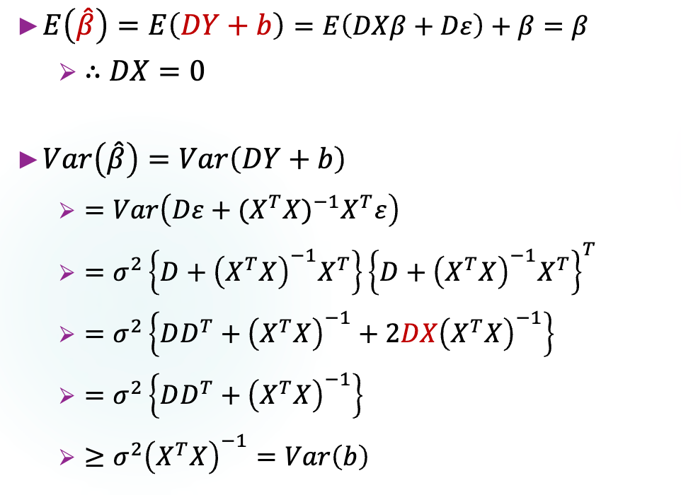
Gauss-Markov Theorem

Under Gauss-Markov assumptions:

1. Linearity: the parameters are themselves linear
2. Randomness: the data must have been randomly sampled from the population
3. Non-Collinearity: the regressors aren’t perfectly correlated with each other
4. Exogeneity: the regressors aren't correlated with the error term, $\mathbb{E}[\varepsilon\mid X]=0$. （给定向量还是给定整个设计矩阵？）
5. Homoscedasticity: no matter what the values of the regressors might be, the error of the variance is constant.
   the OLS estimate for regression coefficients gives you the best linear unbiased estimate (BLUE) possible.

The Leverage

On one hand

$$H^T=H=H^{2}\implies h_{ii}=e_{i}^THe_{i}=e_{i}^TH^THe_{i}\geq 0$$

On the other hand,

$$e_{i}^THe_{i}=h_{ii}=e_{i}^TH^{2}e_{i}=h_{ii}^{2}+\sum _{i\ne j}h_{ij}^{2}\implies h_{ii}\geq h_{ii}^{2}\implies h_{ii}\leq 1$$

In conclusion we have

$$h_{ii}\in [0,1]$$

有时间研究一下取等条件

Don't forget that

$$h_{ii}=\frac{ \partial \hat{Y}_{i} }{ \partial Y_{i} } = \frac{ \partial \sum_{j=1}^{n} h_{ij}Y_{j} }{ \partial Y_{i} }$$

---

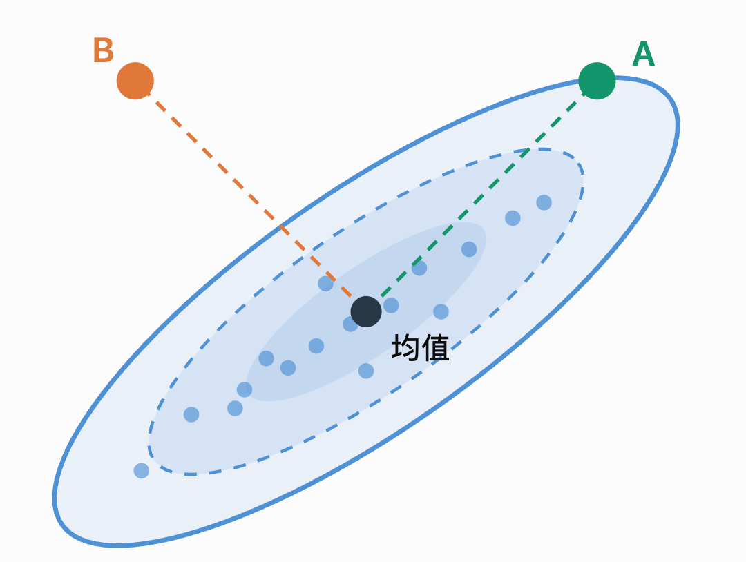
Recall that here we say the leverage describes the distance of $X_{i}$ from the center $\bar{X}$. Now we extend this concept to higher dimension.

The overall principle is to adjust the spread of each direction.

Let $(1, x_{i}^T)$ be the $i$-th row of $X$ and let $\bar{x}=\frac{1}{n}\sum x_{i}$. Here we define the distance of $x_{i}$ from the center $\bar{x}$:

$$D(x_{i},\bar{x})=\sqrt{(x_{i}-\bar{x})^T\Sigma^{-1}(x-\bar{x})}$$

where $\Sigma$ is the sample covariance matrix. Can show that

$$h_{ii}=\frac1n+\frac{D^2(x_{i},\bar{x})}{n-1}$$

▶

The proof

This distance measure is known as Mahalanobis Distance.

Let $X=[\boldsymbol{1}\ Z]$, and $Z_{c}=Z-\frac{1}{n}\boldsymbol{1}\boldsymbol{1}^TZ=(I-J)Z$ (centralize it). Then

$$\Sigma=\frac{1}{n-1}Z_{c}^TZ_{c}=\frac{1}{n-1}Z^T(I-J)Z$$

We hope to find the relationship between the diagonal elements of

$$Z\Sigma^{-1}Z^T\ \text{and}\ H$$

Expand $H$ as

$$[1\ Z]\left( [1\ Z]^T[1\ Z] \right) ^{-1}[1\ Z]^T= [1\ Z] \begin{bmatrix} n & \boldsymbol{1}^TZ \\ Z^T\boldsymbol{1} & Z^TZ \end{bmatrix}^{-1} [1\ Z]^T$$

Recall the knowledge of Shur complement. Shur complement of $n$ is

$$Z^TZ-(Z^T\boldsymbol{1})n^{-1}(\boldsymbol{1}^TZ)=Z^T(I-J)Z=:S$$

it is reversible iff $\boldsymbol{1}\not\in \mathcal{R}(Z)$, which is guaranteed. So

$$\begin{bmatrix} n & \boldsymbol{1}^TZ \\ Z^T\boldsymbol{1} & Z^TZ \end{bmatrix}^{-1} =\begin{bmatrix} \frac1n+\bar z^TS^{-1}\bar z&-\bar z^TS^{-1}\\ -S^{-1}\bar z&S^{-1} \end{bmatrix}$$

therefore

$$h_{ii}= \begin{bmatrix} 1 & z_{i}^T \end{bmatrix} \begin{bmatrix} \frac1n+\bar z^TS^{-1}\bar z&-\bar z^TS^{-1}\\ -S^{-1}\bar z&S^{-1} \end{bmatrix} \begin{bmatrix} 1 \\ z_{i} \end{bmatrix} = \frac{1}{n}+(z_{i}-\bar{z})^TS^{-1}(z_{i}-\bar{z})$$

Note that $S^{-1}=\Sigma^{-1}/(n-1)$, so

$$h_{ii}=\frac{1}{n}+\frac{D^{2}(z_{i},\bar{z})}{n-1}$$

Covariance Matrix of $e$

$$\mathrm{Cov}(e)=\mathrm{Cov}((I-H)Y)=\sigma^{2}(I-H)$$

so

$$\begin{align} \mathrm{Var}(e_{i}) & =\sigma^{2}(1-h_{ii}) \\ \mathrm{Cov}(e_{i},e_{j}) & =-\sigma^{2}h_{ij} \end{align}$$

Think a bit deeper: $h_{ii}$ large $\implies$ $\mathrm{Var}(e_{i})$ closer to 0 $\implies$ fitting is more stable.

Expected Mean Squares and ANOVA F-Test

Already showed that

$$\mathbb{E}[MSE]=\sigma^{2}$$

Let's see $MSR=\frac{\|(H-J)Y\|^{2}}{p-1}$.

$$\begin{align} \mathbb{E}[MSR] & = \frac{1}{p-1}\mathbb{E}[Y^T(H-J)Y] \\ & =\frac{1}{p-1}(\mathrm{Tr}((H-J)\sigma^{2})+(X\beta)^T(H-J)(X\beta)) \\ & = \sigma^{2}+\frac{1}{p-1}(X\beta)^T(H-J)(X\beta) \end{align}$$

Easy to see that

$$(X\beta)^T(H-J)(X\beta)=0 \iff \beta_{1}=\beta_{2}=\dots=\beta_{p-1}=0$$

▶

The proof

Note that $H-J$ is a projection matrix. So

$$(X\beta)^T(H-J)(X\beta)=0 \iff (H-J)X\beta=0$$

Because $X\beta\in \mathcal{R}(H)$ and $\mathcal{R}(H)=\mathcal{R}(H-J)\oplus \mathcal{R}(J)$, we have

$$(H-J)X\beta=0 \iff X\beta\in \mathcal{R}(J)=\mathrm{span}(\boldsymbol{1}) \iff \beta_{2}=\dots=\beta_{p-1}=0$$

This can be used to conduct the F-test:

• $H_{0}:$ $\beta_{1}=\beta_{2}=\dots=\beta_{p-1}=0$.
• $H_{1}:$ $\beta_{k}\ne 0$ for at least one $k$ in $1,2,\dots,p-1$.

The F-statistic is

$$F=\frac{MSR}{MSE}\sim F_{p-1,n-p}$$

Reject $H_{0}$ if $F$ is large enough.

$R^{2}$ and Adjusted $R^{2}$

$$R^{2}=1-\frac{SSE}{SST}$$

But adding regressors can always decrease $SSE$. Penalty on adding regressors needed.

$$R_{a}^{2}=1-\frac{MSE}{MST}=1-\frac{n-1}{\color{red}n-p}\cdot\frac{SSE}{SST}$$