Problem 1 (Neyman’s approach & Regression approach)
a.
This design breaks SUTVA because students in the same classroom can influence each other.
b.
τ ^ d i f = 65.38333 − 50.88333 = 14.5 \hat{\tau}^{\mathrm{dif}}=65.38333-50.88333=14.5 τ ^ dif = 65.38333 − 50.88333 = 14.5
V ^ n e y m a n = 60.597 \hat{\mathbb{V}}^{\mathrm{neyman}}=60.597 V ^ neyman = 60.597
95% CI: 14.5 ± z 0.975 V ^ n e y m a n = ( − 0.76 , 29.76 ) 14.5\pm z_{0.975}\sqrt{\hat{\mathbb{V}}^{\mathrm{neyman}}}=(-0.76,29.76) 14.5 ± z 0.975 V ^ neyman = ( − 0.76 , 29.76 )
There is no enough evidence to reject the null hypothesis of no treatment effect.
c.
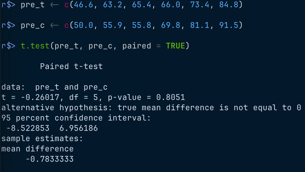
I believe that they were randomly selected because the p-value of the paired t-test is 0.8.
d.
τ ^ d i f = 15.28333 \hat{\tau}^{\mathrm{dif}}=15.28333 τ ^ dif = 15.28333
V ^ n e y m a n = 28.97072 \hat{\mathbb{V}}^{\mathrm{neyman}}=28.97072 V ^ neyman = 28.97072
95% CI: 15.28 ± z 0.975 V ^ n e y m a n = ( 4.73 , 25.82 ) 15.28\pm z_{0.975}\sqrt{\hat{\mathbb{V}}^{\mathrm{neyman}}}=(4.73,25.82) 15.28 ± z 0.975 V ^ neyman = ( 4.73 , 25.82 )
There is enough evidence to reject the null hypothesis of no treatment effect.
e.
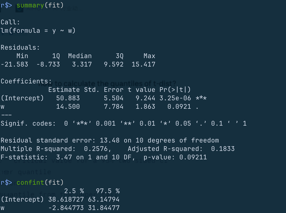
The results are the same as (b) because I used V ^ n e y m a n \hat{\mathbb{V}}^{\mathrm{neyman}} V ^ neyman
f.
g.
p.s.
s t 2 6 + s c 2 6 = 60.59722 1 10 ( 5 s t 2 + 5 s c 2 ) ( 1 6 + 1 6 ) = 60.59722 \begin{aligned}
\frac{s_{t}^{2}}{6}+\frac{s_{c}^{2}}{6} & =60.59722 \\
\frac{1}{10}(5s_{t}^{2}+5s_{c}^{2})\left( \frac{1}{6}+\frac{1}{6} \right) & = 60.59722
\end{aligned}
6 s t 2 + 6 s c 2 10 1 ( 5 s t 2 + 5 s c 2 ) ( 6 1 + 6 1 ) = 60.59722 = 60.59722
That's why the CI is the same as that in (f).
h.
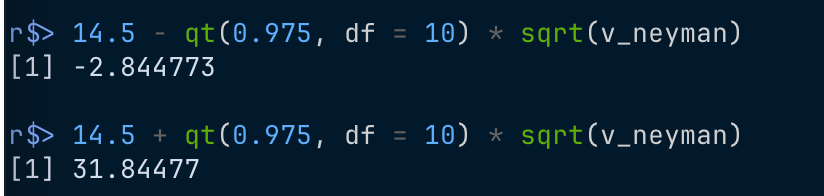
(b) and (e) are the same. (f) is different because it uses t-distribution to construct the CI. Replacing z 0.975 z_{0.975} z 0.975 t 0.975 , 10 t_{0.975,10} t 0.975 , 10
Problem 2 (Theory for Neyman's approach)
(1)
a.
τ ^ d i f = ∑ Y i ( 1 ) W i ∑ W i − ∑ Y i ( 0 ) ( 1 − W i ) ∑ ( 1 − W i ) \hat{\tau}^{\mathrm{dif}}=\frac{\sum Y_{i}(1)W_i}{\sum W_i}- \frac{\sum Y_{i}(0)(1-W_i)}{\sum(1-W_i)}
τ ^ dif = ∑ W i ∑ Y i ( 1 ) W i − ∑ ( 1 − W i ) ∑ Y i ( 0 ) ( 1 − W i )
b.
Under complete randomization, W i W_i W i
E [ W i ] = N t N ∑ W i = N t \mathbb{E}[W_i]=\frac{N_t}{N}\quad \sum W_i=N_t
E [ W i ] = N N t ∑ W i = N t
therefore
E [ τ ^ d i f ] = ∑ Y i ( 1 ) N t N N t − ∑ Y i ( 0 ) N c N N c = τ f s \mathbb{E}[\hat{\tau}^{\mathrm{dif}}]=\frac{\sum Y_{i}(1) \frac{N_t}{N}}{N_t}-\frac{\sum Y_{i}(0) \frac{N_c}{N}}{N_c}=\tau_{fs}
E [ τ ^ dif ] = N t ∑ Y i ( 1 ) N N t − N c ∑ Y i ( 0 ) N N c = τ f s
c.
τ ^ d i f = 1 N t ∑ i : W i = 1 ( Y i o b s − X i ) − 1 N c ∑ i : W i = 0 ( Y i o b s − X i ) = ∑ ( Y i ( 1 ) − X i ) W i ∑ W i − ∑ ( Y i ( 0 ) − X i ) ( 1 − W i ) ∑ ( 1 − W i ) \begin{aligned}
\hat{\tau}^{\mathrm{dif}} & = \frac{1}{N_t}\sum_{i:W_i=1}(Y_i^{obs}-X_{i})-\frac{1}{N_c}\sum_{i:W_i=0}(Y_i^{obs}-X_{i}) \\
& = \frac{\sum(Y_{i}(1)-X_{i})W_{i}}{\sum W_{i}}-\frac{\sum(Y_{i}(0)-X_{i})(1-W_{i})}{\sum (1-W_{i})}
\end{aligned}
τ ^ dif = N t 1 i : W i = 1 ∑ ( Y i o b s − X i ) − N c 1 i : W i = 0 ∑ ( Y i o b s − X i ) = ∑ W i ∑ ( Y i ( 1 ) − X i ) W i − ∑ ( 1 − W i ) ∑ ( Y i ( 0 ) − X i ) ( 1 − W i )
d.
Similar to (b)
E [ τ ^ d i f ] = 1 N ∑ ( Y i ( 1 ) − X i ) − 1 N ∑ ( Y i ( 0 ) − X i ) = τ f s \mathbb{E}[\hat{\tau}^{\mathrm{dif}}]=\frac{1}{N}\sum(Y_{i}(1)-X_i)-\frac{1}{N}\sum(Y_{i}(0)-X_i)=\tau_{fs}
E [ τ ^ dif ] = N 1 ∑ ( Y i ( 1 ) − X i ) − N 1 ∑ ( Y i ( 0 ) − X i ) = τ f s
e.
They have different variances.
(2)
E [ Y i o b s ( X i − μ X ) ] = E { [ Y i ( 1 ) W i + Y i ( 0 ) ( 1 − W i ) ] X i } − μ X E [ Y i ( 1 ) W i + Y i ( 0 ) ( 1 − W i ) ] \mathbb{E}[Y_{i}^{obs}(X_i-\mu_X)]=\mathbb{E}\left\{ [Y_{i}(1)W_i+Y_i(0)(1-W_i)]X_{i} \right\}-\mu_{X}\mathbb{E}[Y_{i}(1)W_i+Y_i(0)(1-W_i)]
E [ Y i o b s ( X i − μ X )] = E { [ Y i ( 1 ) W i + Y i ( 0 ) ( 1 − W i )] X i } − μ X E [ Y i ( 1 ) W i + Y i ( 0 ) ( 1 − W i )]
The former part:
… = E [ X i Y i ( 1 ) N t N + X i Y i ( 0 ) N c N ] = N t N ( C o v ( X i , Y i ( 1 ) ) + μ X μ t ) + N c N ( C o v ( X i , Y i ( 0 ) ) + μ X μ c ) \begin{aligned}
\dots & = \mathbb{E}\left[ X_iY_i(1) \frac{N_{t}}{N}+X_iY_i(0) \frac{N_c}{N} \right] \\
& = \frac{N_{t}}{N}(\mathrm{Cov}(X_{i},Y_{i}(1))+\mu_{X}\mu_{t})+\frac{N_c}{N}(\mathrm{Cov}(X_{i},Y_{i}(0))+\mu_{X}\mu_{c})
\end{aligned}
… = E [ X i Y i ( 1 ) N N t + X i Y i ( 0 ) N N c ] = N N t ( Cov ( X i , Y i ( 1 )) + μ X μ t ) + N N c ( Cov ( X i , Y i ( 0 )) + μ X μ c )
The later part:
… = μ X ( μ t N t N + μ c N c N ) \begin{aligned}
\dots & = \mu_{X}\left( \mu_{t} \frac{N_t}{N}+\mu_{c} \frac{N_c}{N} \right)
\end{aligned}
… = μ X ( μ t N N t + μ c N N c )
thus
E [ Y i o b s ( X i − μ X ) ] = N t N C o v ( X i , Y ( 1 ) ) + N c N C o v ( X i , Y i ( 0 ) ) \mathbb{E}[Y_{i}^{obs}(X_i-\mu_X)]=\frac{N_t}{N}\mathrm{Cov}(X_i,Y(1))+ \frac{N_c}{N}\mathrm{Cov}(X_i,Y_i(0))
E [ Y i o b s ( X i − μ X )] = N N t Cov ( X i , Y ( 1 )) + N N c Cov ( X i , Y i ( 0 ))
Problem 3 (Theory for Regression approach)
a.
1 N ∑ i = 1 N τ ^ i = 1 N [ ∑ i : W i = 1 ( Y i ( 1 ) − Y ˉ c ) + ∑ i : W i = 0 ( Y ˉ t − Y i ( 0 ) ) ] = 1 N ( N t Y ˉ t − N t Y ˉ c + N c Y ˉ t − N c Y ˉ c ) = Y ˉ t − Y ˉ c = τ ^ d i f \begin{aligned}
\frac{1}{N}\sum_{i=1}^{N} \hat{\tau}_{i} & = \frac{1}{N}\left[ \sum _{i:W_i=1}(Y_{i}(1)-\bar{Y}_{c})+\sum _{i:W_i=0}(\bar{Y}_{t}-Y_{i}(0)) \right] \\
& = \frac{1}{N}(N_{t}\bar{Y}_{t}-N_{t}\bar{Y}_{c}+N_{c}\bar{Y}_{t}-N_{c}\bar{Y}_{c}) \\
& = \bar{Y}_{t}-\bar{Y}_{c} \\
& = \hat{\tau}^{\mathrm{dif}}
\end{aligned}
N 1 i = 1 ∑ N τ ^ i = N 1 [ i : W i = 1 ∑ ( Y i ( 1 ) − Y ˉ c ) + i : W i = 0 ∑ ( Y ˉ t − Y i ( 0 )) ] = N 1 ( N t Y ˉ t − N t Y ˉ c + N c Y ˉ t − N c Y ˉ c ) = Y ˉ t − Y ˉ c = τ ^ dif
b.
Let τ i = Y i ( 1 ) − Y i ( 0 ) , E [ Y 1 ( 1 ) ] = μ t , E [ Y i ( 0 ) ] = μ c , E [ τ i ] = τ s p , E [ W i ] = p \tau_{i}=Y_i(1)-Y_i(0),\mathbb{E}[Y_1(1)]=\mu_{t},\mathbb{E}[Y_i(0)]=\mu_{c},\mathbb{E}[\tau_{i}]=\tau_{sp},\mathbb{E}[W_i]=p τ i = Y i ( 1 ) − Y i ( 0 ) , E [ Y 1 ( 1 )] = μ t , E [ Y i ( 0 )] = μ c , E [ τ i ] = τ s p , E [ W i ] = p
E [ ( Y i o b s − α − τ W i ) 2 ] = E [ ( ( τ i − τ ) W i + Y i ( 0 ) − α ) 2 ] = p [ E ( τ i − τ s p ) 2 + ( τ s p − τ ) 2 ] + E [ ( Y i ( 0 ) − μ c ) 2 ] + ( μ c − α ) 2 + 2 p E ( τ i − τ ) ( Y i ( 0 ) − α ) = … = p τ 2 + α 2 + 2 p τ α − 2 p μ t τ − 2 ( μ c + p τ s p ) α + … \begin{aligned}
\mathbb{E}[(Y_{i}^{obs}-\alpha-\tau W_{i})^{2}] & = \mathbb{E}[((\tau_{i}-\tau)W_i+Y_i(0)-\alpha)^{2}] \\
& = p[\mathbb{E}(\tau_{i}-\tau_{sp})^{2}+(\tau_{sp}-\tau)^{2}] \\
& +\mathbb{E}[(Y_i(0)-\mu_{c})^{2}]+ (\mu_{c}-\alpha)^{2} \\
& +2p\mathbb{E}(\tau_{i}-\tau)(Y_{i}(0)-\alpha) \\
& = \dots \\
& = p\tau^{2}+\alpha^{2}+2p\tau \alpha-2p\mu_{t}\tau-2(\mu_{c}+p\tau_{sp})\alpha+\dots
\end{aligned}
E [( Y i o b s − α − τ W i ) 2 ] = E [(( τ i − τ ) W i + Y i ( 0 ) − α ) 2 ] = p [ E ( τ i − τ s p ) 2 + ( τ s p − τ ) 2 ] + E [( Y i ( 0 ) − μ c ) 2 ] + ( μ c − α ) 2 + 2 p E ( τ i − τ ) ( Y i ( 0 ) − α ) = … = p τ 2 + α 2 + 2 p τ α − 2 p μ t τ − 2 ( μ c + p τ s p ) α + …
the "..." in the last line has nothing to do with ( α , τ ) (\alpha,\tau) ( α , τ ) p τ 2 + α 2 + 2 p τ α − 2 p μ t τ − 2 ( μ c + p τ s p ) α p\tau^{2}+\alpha^{2}+2p\tau \alpha-2p\mu_{t}\tau-2(\mu_{c}+p\tau_{sp})\alpha p τ 2 + α 2 + 2 p τ α − 2 p μ t τ − 2 ( μ c + p τ s p ) α
Apparently it has minimum. Find its first order conditions:
τ + α = μ t α − μ c = p ( τ s p − τ ) \begin{aligned}
\tau+\alpha & =\mu_{t} \\
\alpha-\mu_{c} & =p(\tau_{sp}-\tau)
\end{aligned}
τ + α α − μ c = μ t = p ( τ s p − τ )
The solution is
α = μ c τ = τ s p \begin{aligned}
\alpha & = \mu_{c} \\
\tau & =\tau_{sp}
\end{aligned}
α τ = μ c = τ s p
There is a more elegant way:
E [ ( Y i o b s − α − τ W i ) 2 ] = p E [ ( Y i ( 1 ) − α − τ ) 2 ] + ( 1 − p ) E [ ( Y i ( 0 ) − α ) 2 ] = p E [ ( Y i ( 1 ) − μ t + μ t − α − τ ) 2 ] + ( 1 − p ) E [ ( Y i ( 0 ) − μ c + μ c − α ) 2 ] = p [ σ t 2 + ( μ t − α − τ ) 2 ] + ( 1 − p ) [ σ c 2 + ( μ c − α 2 ) ] \begin{aligned}
\mathbb{E}[(Y_{i}^{obs}-\alpha-\tau W_{i})^{2}] & = p\mathbb{E}[(Y_{i}(1)-\alpha-\tau)^{2}]+(1-p)\mathbb{E}[(Y_{i}(0)-\alpha)^{2}] \\
& = p\mathbb{E}[(Y_{i}(1)-\mu_{t}+\mu_{t}-\alpha-\tau)^{2}]+(1-p)\mathbb{E}[(Y_{i}(0)-\mu_{c}+\mu_{c}-\alpha)^{2}] \\
& = p[\sigma_{t}^{2}+(\mu_{t}-\alpha-\tau)^{2}]+(1-p)[\sigma_{c}^{2}+(\mu_{c}-\alpha^{2})]
\end{aligned}
E [( Y i o b s − α − τ W i ) 2 ] = p E [( Y i ( 1 ) − α − τ ) 2 ] + ( 1 − p ) E [( Y i ( 0 ) − α ) 2 ] = p E [( Y i ( 1 ) − μ t + μ t − α − τ ) 2 ] + ( 1 − p ) E [( Y i ( 0 ) − μ c + μ c − α ) 2 ] = p [ σ t 2 + ( μ t − α − τ ) 2 ] + ( 1 − p ) [ σ c 2 + ( μ c − α 2 )]
The first line uses
Law of total expectation
W i ⊥ ( Y i ( 1 ) , Y i ( 0 ) ) W_i\perp (Y_i(1),Y_i(0)) W i ⊥ ( Y i ( 1 ) , Y i ( 0 ))
The second line means to get the variances.