The two experiments introduced below are aimed to get unbiased estimators with less variance.
Stratified Randomized Experiment
Notations
Group the data into J J J
Implement a CRE within each data strata
In each stratum j j j N ( j ) , N c ( j ) , N t ( j ) N(j),N_{c}(j),N_{t}(j) N ( j ) , N c ( j ) , N t ( j )
Proportion of stratum j j j q ( j ) = N ( j ) / N q(j)=N(j)/N q ( j ) = N ( j ) / N Propensity score of stratum j j j e ( j ) = N t ( j ) / N ( j ) e(j)=N_{t}(j)/N(j) e ( j ) = N t ( j ) / N ( j )
Let G i G_{i} G i i i i B i ( j ) = 1 ( G i = j ) B_{i}(j)=\mathbb{1}(G_{i}=j) B i ( j ) = 1 ( G i = j )
The assignment mechanism:
P ( W ∣ X , Y ( 0 ) , Y ( 1 ) ) = ∏ j = 1 J ( N ( j ) N t ( j ) ) − 1 for reasonable W , 0 for others P(\boldsymbol{W}\mid \boldsymbol{X},\boldsymbol{Y}(0),\boldsymbol{Y}(1))=\prod_{j=1}^{J} \binom{N(j)}{N_{t}(j)}^{-1} \text{for reasonable}\ \boldsymbol{W}, 0\ \text{for others}
P ( W ∣ X , Y ( 0 ) , Y ( 1 )) = j = 1 ∏ J ( N t ( j ) N ( j ) ) − 1 for reasonable W , 0 for others
Also known as Randomized Blocks Experiments (RBEs).
Causal Estimands in SREs
Take a two-stratum example, male and female.
τ f s ( f ) = 1 N ( f ) ∑ i : G i = f ( Y i ( 1 ) − Y i ( 0 ) ) \tau_{fs}(f)=\frac{1}{N(f)}\sum _{i:G_{i}=f}\left( Y_{i}(1)-Y_{i}(0) \right)
τ f s ( f ) = N ( f ) 1 i : G i = f ∑ ( Y i ( 1 ) − Y i ( 0 ) )
τ f s ( m ) = 1 N ( m ) ∑ i : G i = m ( Y i ( 1 ) − Y i ( 0 ) ) \tau_{fs}(m)=\frac{1}{N(m)}\sum _{i:G_{i}=m}\left( Y_{i}(1)-Y_{i}(0) \right)
τ f s ( m ) = N ( m ) 1 i : G i = m ∑ ( Y i ( 1 ) − Y i ( 0 ) )
ACE in all units (weighted average)
τ f s = 1 N ∑ i = 1 N ( Y i ( 1 ) − Y i ( 0 ) ) = q ( f ) ⋅ τ f s ( f ) + q ( m ) ⋅ τ f s ( m ) \tau_{fs}=\frac{1}{N}\sum_{i=1}^{N} \left( Y_{i}(1)-Y_{i}(0) \right) = q(f)\cdot\tau_{fs}(f)+q(m)\cdot\tau_{fs}(m)
τ f s = N 1 i = 1 ∑ N ( Y i ( 1 ) − Y i ( 0 ) ) = q ( f ) ⋅ τ f s ( f ) + q ( m ) ⋅ τ f s ( m )
Inference Approaches for SREs
Still use the example above.
Fisher's Exact P-Values
Keep in mind the purpose of hypothesis testing: to check if the observed data is extreme under H 0 H_{0} H 0
Fisher's sharp null hypothesis:
H 0 : Y i ( 0 ) = Y i ( 1 ) for all i H_{0}: Y_{i}(0)=Y_{i}(1)\ \text{for all}\ i
H 0 : Y i ( 0 ) = Y i ( 1 ) for all i
Choices of test statistics:
T d i f = ∣ Y ˉ t o b s − Y ˉ c o b s ∣ T^{\mathrm{dif}}=\left| \bar{Y}_{t}^{\mathrm{obs}}-\bar{Y}_{c}^{\mathrm{obs}} \right| T dif = Y ˉ t obs − Y ˉ c obs
valid
Not good because under H 0 H_{0} H 0
T d i f , λ = ∣ λ ⋅ ( Y ˉ t o b s ( f ) − Y ˉ c o b s ( f ) ) + ( 1 − λ ) ⋅ ( Y ˉ t o b s ( m ) − Y ˉ c o b s ( m ) ) ∣ T^{\mathrm{dif},\lambda}=\left| \lambda\cdot(\bar{Y}_{t}^{\mathrm{obs}}(f)-\bar{Y}_{c}^{\mathrm{obs}}(f))+(1-\lambda)\cdot(\bar{Y}_{t}^{\mathrm{obs}}(m)-\bar{Y}_{c}^{\mathrm{obs}}(m)) \right| T dif , λ = λ ⋅ ( Y ˉ t obs ( f ) − Y ˉ c obs ( f )) + ( 1 − λ ) ⋅ ( Y ˉ t obs ( m ) − Y ˉ c obs ( m ))
valid
Choosing a good λ \lambda λ q ( f ) q(f) q ( f )
And two rank statistics
But the rank statistics here have lower power compared with CRE due to few outliers in the space of class.
Neyman's Approach
The estimator:
τ ^ s t r a t = q ( f ) ⋅ τ ^ d i f ( f ) + q ( m ) ⋅ τ ^ d i f ( m ) \hat{\tau}^{\mathrm{strat}}= q(f)\cdot\hat{\tau}^{\mathrm{dif}}(f)+q(m)\cdot\hat{\tau}^{\mathrm{dif}}(m)
τ ^ strat = q ( f ) ⋅ τ ^ dif ( f ) + q ( m ) ⋅ τ ^ dif ( m )
The estimator's expectation and variance can be deduced:
E W [ τ ^ s t r a t ] = q ( f ) ⋅ τ f s ( f ) + q ( m ) ⋅ τ f s ( m ) = τ f s V W ( τ ^ s t r a t ) = q ( f ) 2 V W ( τ ^ f d i f ) + q ( m ) 2 V W ( τ ^ m d i f ) + q ( f ) q ( m ) C o v ( ⋅ , ⋅ ) = q ( f ) 2 V W ( τ ^ f d i f ) + q ( m ) 2 V W ( τ ^ m d i f ) ( τ ^ f d i f and τ ^ m d i f are independent ) \begin{align} \mathbb{E}_{W}[\hat{\tau}^{\mathrm{strat}}] & =q(f)\cdot\tau_{fs}(f)+q(m)\cdot\tau_{fs}(m)=\tau_{fs} \\ \mathbb{V}_{W}(\hat{\tau}^{\mathrm{strat}}) & =q(f)^{2}\mathbb{V}_{W}(\hat{\tau}^{\mathrm{dif}}_{f})+q(m)^{2}\mathbb{V}_{W}(\hat{\tau}^{\mathrm{dif}}_{m})+q(f)q(m)\mathrm{Cov}(\cdot,\cdot) \\ & = q(f)^{2}\mathbb{V}_{W}(\hat{\tau}^{\mathrm{dif}}_{f})+q(m)^{2}\mathbb{V}_{W}(\hat{\tau}^{\mathrm{dif}}_{m})\quad (\hat{\tau}^{\mathrm{dif}}_{f}\ \text{and}\ \hat{\tau}^{\mathrm{dif}}_{m}\ \text{are independent}) \\ \end{align} E W [ τ ^ strat ] V W ( τ ^ strat ) = q ( f ) ⋅ τ f s ( f ) + q ( m ) ⋅ τ f s ( m ) = τ f s = q ( f ) 2 V W ( τ ^ f dif ) + q ( m ) 2 V W ( τ ^ m dif ) + q ( f ) q ( m ) Cov ( ⋅ , ⋅ ) = q ( f ) 2 V W ( τ ^ f dif ) + q ( m ) 2 V W ( τ ^ m dif ) ( τ ^ f dif and τ ^ m dif are independent )
where the expression of V W ( τ ^ f d i f ) , V W ( τ ^ m d i f ) \mathbb{V}_{W}(\hat{\tau}^{\mathrm{dif}}_{f}),\mathbb{V}_{W}(\hat{\tau}^{\mathrm{dif}}_{m}) V W ( τ ^ f dif ) , V W ( τ ^ m dif ) here .
The estimator Y ˉ t o b s − Y ˉ c o b s \bar{Y}^{\mathrm{obs}}_{t}-\bar{Y}^{\mathrm{obs}}_{c} Y ˉ t obs − Y ˉ c obs
SREs vs CREs
We compare the super-population variances of CRE and SRE under two sampling designs.
For CRE , individuals are independently sampled from the super-population, where P ( G i = f ) = q P(G_{i}=f)=q P ( G i = f ) = q p p p N t / N = p N_{t}/N=p N t / N = p τ ^ d i f \hat{\tau}^{\mathrm{dif}} τ ^ dif
For SRE , we use stratified sampling with fixed stratum proportion q = N ( f ) / N q=N(f)/N q = N ( f ) / N p p p τ ^ s t r a t \hat{\tau}^{\mathrm{strat}} τ ^ strat
Recall Neyman estimator for CRE:
τ ^ d i f = Y ˉ t o b s − Y ˉ c o b s \hat{\tau}^{\mathrm{dif}}=\bar{Y}^{\mathrm{obs}}_{t}-\bar{Y}^{\mathrm{obs}}_{c}
τ ^ dif = Y ˉ t obs − Y ˉ c obs
with super population variance
V s p ( τ ^ d i f ) = σ c 2 N c + σ t 2 N t \mathbb{V}_{sp}(\hat{\tau}^{\mathrm{dif}})=\frac{\sigma_{c}^{2}}{N_{c}}+\frac{\sigma^{2}_{t}}{N_{t}}
V s p ( τ ^ dif ) = N c σ c 2 + N t σ t 2
In order to compare it with SRE, we can divide σ c 2 \sigma_{c}^{2} σ c 2
q σ c 2 ( f ) + ( 1 − q ) σ c 2 ( m ) + q ( 1 − q ) [ μ c ( f ) − μ c ( m ) ] 2 q\sigma_{c}^{2}(f)+(1-q)\sigma_{c}^{2}(m)+q(1-q)[\mu_{c}(f)-\mu_{c}(m)]^{2}
q σ c 2 ( f ) + ( 1 − q ) σ c 2 ( m ) + q ( 1 − q ) [ μ c ( f ) − μ c ( m ) ] 2
by the total variance formula. Similarly σ t 2 \sigma_{t}^{2} σ t 2
Within each stratum, there is a CRE, so
V s p [ τ ^ d i f ( f ) ] = … , V s p [ τ ^ d i f ( m ) ] = … \mathbb{V}_{sp}[\hat{\tau}^{\mathrm{dif}}(f)]=\dots,\ \mathbb{V}_{sp}[\hat{\tau}^{\mathrm{dif}}(m)]=\dots
V s p [ τ ^ dif ( f )] = … , V s p [ τ ^ dif ( m )] = …
and τ ^ d i f ( f ) ⊥ τ ^ d i f ( m ) \hat{\tau}^{\mathrm{dif}}(f)\perp \hat{\tau}^{\mathrm{dif}}(m) τ ^ dif ( f ) ⊥ τ ^ dif ( m )
Therefore
V s p [ τ ^ s t r a t ] = V s p [ q ⋅ + ( 1 − q ) ⋅ ] = q 2 V s p [ ⋅ ] + ( 1 − q ) 2 V s p [ ⋅ ] = q N ( σ t 2 ( f ) p + σ c 2 ( f ) 1 − p ) + 1 − q N ( σ t 2 ( m ) p + σ c 2 ( m ) 1 − p ) \begin{align}
\mathbb{V}_{sp}[\hat{\tau}^{\mathrm{strat}}] & = \mathbb{V}_{sp}[q\cdot+(1-q)\cdot] \\
& = q^{2}\mathbb{V}_{sp}[\cdot]+(1-q)^{2}\mathbb{V}_{sp}[\cdot] \\
& = \frac{q}{N}\left( \frac{\sigma_{t}^{2}(f)}{p}+\frac{\sigma_{c}^{2}(f)}{1-p} \right) + \frac{1-q}{N}\left( \frac{\sigma^{2}_{t}(m)}{p}+ \frac{\sigma^{2}_{c}(m)}{1-p}\right)
\end{align}
V s p [ τ ^ strat ] = V s p [ q ⋅ + ( 1 − q ) ⋅ ] = q 2 V s p [ ⋅ ] + ( 1 − q ) 2 V s p [ ⋅ ] = N q ( p σ t 2 ( f ) + 1 − p σ c 2 ( f ) ) + N 1 − q ( p σ t 2 ( m ) + 1 − p σ c 2 ( m ) )
where σ t 2 ( f ) = V s p [ Y i ( 1 ) ∣ G i = f ] , … \sigma_{t}^{2}(f)=\mathbb{V}_{sp}[Y_{i}(1)\mid G_{i}=f],\dots σ t 2 ( f ) = V s p [ Y i ( 1 ) ∣ G i = f ] , …
Can verify that
V s p [ τ ^ d i f ] − V s p [ τ ^ s t r a t ] = q ( 1 − q ) ⋅ [ ( μ c ( f ) − μ c ( m ) ) 2 N ( 1 − p ) + ( μ t ( f ) − μ t ( m ) ) 2 N p ] ≥ 0 \mathbb{V}_{sp}[\hat{\tau}^{\mathrm{dif}}]-\mathbb{V}_{sp}[\hat{\tau}^{\mathrm{strat}}]=q(1-q)\cdot\left[ \frac{(\mu_{c}(f)-\mu_{c}(m))^{2}}{N(1-p)}+\frac{(\mu_{t}(f)-\mu_{t}(m))^{2}}{Np} \right]\geq 0
V s p [ τ ^ dif ] − V s p [ τ ^ strat ] = q ( 1 − q ) ⋅ [ N ( 1 − p ) ( μ c ( f ) − μ c ( m ) ) 2 + N p ( μ t ( f ) − μ t ( m ) ) 2 ] ≥ 0
One is never worse off stratifying on a covariate. The gain in precision comes from the prediction capability of the stratification.
That is saying that if the stratification does have the ability to distinguish the potential outcomes, than the gain in precision is good. We fully utilized the information.
Regression Analysis of SREs
Keep in mind that the estimand is
τ s p = E [ Y i ( 1 ) − Y i ( 0 ) ] = ∑ j = 1 J q ( j ) τ s p ( j ) \begin{align}
\tau_{sp} & =\mathbb{E}[Y_{i}(1)-Y_{i}(0)] \\
& = \sum_{j=1}^{J} q(j)\tau_{sp}(j)
\end{align}
τ s p = E [ Y i ( 1 ) − Y i ( 0 )] = j = 1 ∑ J q ( j ) τ s p ( j )
Where q ( j ) = P ( B i ( j ) = 1 ) q(j)=P(B_{i}(j)=1) q ( j ) = P ( B i ( j ) = 1 ) N ( j ) / N N(j)/N N ( j ) / N
The following model is the real one, we should directly estimate this one. I think the section "Without Interaction" is nonsense. Why do we have to discuss it?
Without Interaction
Regression model:
Y i o b s = τ W i + ∑ j = 1 J β ( j ) B i ( j ) + ε i Y_i^{\mathrm{obs}}=\tau W_i+\sum_{j=1}^{J}\beta(j)B_i(j)+\varepsilon_i
Y i obs = τ W i + j = 1 ∑ J β ( j ) B i ( j ) + ε i
Least square estimate:
( τ ^ o l s , β ^ o l s ) = argmin τ , β ∑ i = 1 N ( … ) 2 (\hat{\tau}^{ol s},\hat{\beta}^{ol s})=\operatorname*{argmin}_{\tau,\beta}\sum_{i=1}^{N} (\dots)^{2}
( τ ^ o l s , β ^ o l s ) = τ , β argmin i = 1 ∑ N ( … ) 2
Population counterparts to these OLS:
( τ ∗ , β ∗ ) = argmin τ , β E [ ( … ) 2 ] (\tau^{*},\beta^{*})=\operatorname*{argmin}_{\tau,\beta}\mathbb{E}[ (\dots)^{2}]
( τ ∗ , β ∗ ) = τ , β argmin E [( … ) 2 ]
Suppose we conduct a stratified randomized experiment in a sample drawn at random from an infinite population. Then
τ ∗ = τ ω \tau^{*}=\tau_{\omega} τ ∗ = τ ω τ ω = ∑ j = 1 J ω ( j ) τ s p ( j ) / ( ∑ j = 1 J ω ( j ) ) , ω ( j ) = q ( j ) e ( j ) ( 1 − e ( j ) ) \tau_{\omega}=\sum_{j=1}^{J} \omega(j)\tau_{sp}(j)\big/ \left( \sum_{j=1}^{J} \omega(j) \right),\ \omega(j)=q(j)e(j)(1-e(j)) τ ω = j = 1 ∑ J ω ( j ) τ s p ( j ) / ( j = 1 ∑ J ω ( j ) ) , ω ( j ) = q ( j ) e ( j ) ( 1 − e ( j ))
N ⋅ ( τ ^ ols − τ ω ) → d N ( 0 , E [ ( W i − ∑ j = 1 J q ( j ) ⋅ B i ( j ) ) 2 ⋅ ( Y i obs − τ ∗ ⋅ W i − ∑ j = 1 J β j ∗ ⋅ B i ( j ) ) 2 ] ( ∑ j = 1 J q ( j ) ⋅ e ( j ) ⋅ ( 1 − e ( j ) ) ) 2 ) \sqrt{N} \cdot \left( \hat{\tau}^{\text{ols}} - \tau_{\omega} \right) \xrightarrow{d} \mathcal{N} \left( 0, \frac{\mathbb{E}\left[ \left( W_i - \sum_{j=1}^{J} q(j) \cdot B_i(j) \right)^2 \cdot \left( Y_i^{\text{obs}} - \tau^* \cdot W_i - \sum_{j=1}^{J} \beta_j^* \cdot B_i(j) \right)^2 \right]}{\left( \sum_{j=1}^{J} q(j) \cdot e(j) \cdot (1 - e(j)) \right)^2} \right) N ⋅ ( τ ^ ols − τ ω ) d N ( 0 , ( ∑ j = 1 J q ( j ) ⋅ e ( j ) ⋅ ( 1 − e ( j )) ) 2 E [ ( W i − ∑ j = 1 J q ( j ) ⋅ B i ( j ) ) 2 ⋅ ( Y i obs − τ ∗ ⋅ W i − ∑ j = 1 J β j ∗ ⋅ B i ( j ) ) 2 ] )
Note that τ ω \tau_{\omega} τ ω τ s p \tau_{sp} τ s p
e ( j ) e(j) e ( j ) τ s p ( j ) \tau_{sp}(j) τ s p ( j )
Adding Interactions
The model is
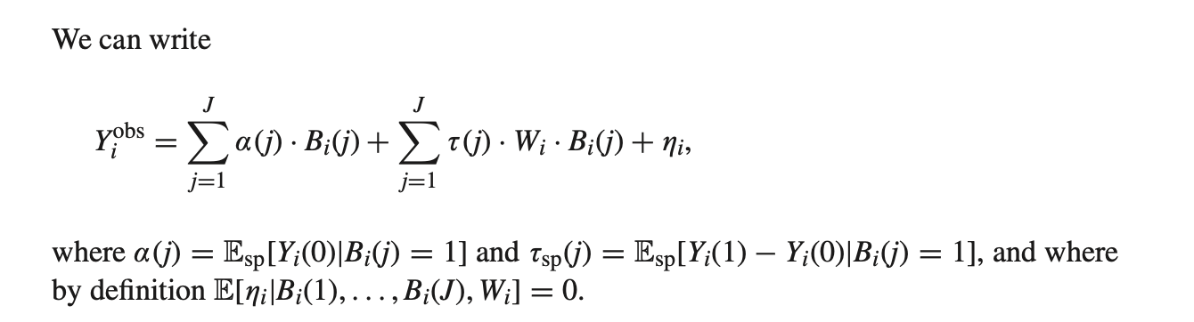
Y i o b s = ∑ j = 1 J β j B i ( j ) + ∑ j = 1 J τ j W i B i ( j ) + ε i Y_i^{obs} =\sum_{j=1}^J\beta_j B_i(j) +\sum_{j=1}^J\tau_j W_i B_i(j) +\varepsilon_i
Y i o b s = j = 1 ∑ J β j B i ( j ) + j = 1 ∑ J τ j W i B i ( j ) + ε i
which allows each stratum has its own intersection and treatment effect. Having gotten τ ^ j \hat{\tau}_{j} τ ^ j τ ^ s t r a t \hat{\tau}^{\mathrm{strat}} τ ^ strat
Y i o b s = ∑ j = 1 J β ( j ) B i ( j ) + τ W i B i ( J ) q ( J ) + ∑ j = 1 J − 1 γ ( j ) W i ( B i ( j ) − q ( j ) q ( J ) B i ( J ) ) + ε i Y_i^{obs} =\sum_{j=1}^J\beta(j)B_i(j) +\tau W_i\frac{B_i(J)}{q(J)}+\sum_{j=1}^{J-1}\gamma(j)W_i \left(B_i(j)-\frac{q(j)}{q(J)}B_i(J)\right) +\varepsilon_i
Y i o b s = j = 1 ∑ J β ( j ) B i ( j ) + τ W i q ( J ) B i ( J ) + j = 1 ∑ J − 1 γ ( j ) W i ( B i ( j ) − q ( J ) q ( j ) B i ( J ) ) + ε i
Use a simple example to catch the essence of the rewriting: suppose we have the model
Y = β 0 + β 1 X 1 + β 2 X 2 + ε Y=\beta_{0}+\beta_{1}X_{1}+\beta_{2}X_{2}+\varepsilon Y = β 0 + β 1 X 1 + β 2 X 2 + ε
And we want to estimate a β 1 + b β 2 a\beta_{1}+b\beta_{2} a β 1 + b β 2
Y = β 0 + ( a β 1 + b β 2 ) X 1 a + β 2 ( X 2 − b a X 1 ) + ε Y=\beta_{0}+(a\beta_{1}+b\beta_{2}) \frac{X_{1}}{a}+\beta_{2}\left( X_{2}-\frac{b}{a}X_{1} \right)+\varepsilon Y = β 0 + ( a β 1 + b β 2 ) a X 1 + β 2 ( X 2 − a b X 1 ) + ε
More generally,
Y = β T X + ε = ( A β ) T ( A − 1 X ) + ε Y=\beta^TX+\varepsilon=(A\beta)^T(A^{-1}X)+\varepsilon Y = β T X + ε = ( A β ) T ( A − 1 X ) + ε
Least square estimate: τ ^ o l s , i n t e r \hat{\tau}^{ol s,inter} τ ^ o l s , in t er τ ∗ \tau^{*} τ ∗
Suppose we conduct a stratified randomized experiment in a sample drawn at random from an infinite population. Then
τ ∗ = τ sp \tau^* = \tau_{\text{sp}} τ ∗ = τ sp N ⋅ ( τ ^ ols,inter − τ sp ) → d N ( 0 , ∑ j = 1 J q ( j ) 2 ⋅ ( σ c 2 ( j ) ( 1 − e ( j ) ) ⋅ q ( j ) + σ t 2 ( j ) e ( j ) ⋅ q ( j ) ) ) \sqrt{N} \cdot \left( \hat{\tau}^{\text{ols,inter}} - \tau_{\text{sp}} \right) \xrightarrow{d} \mathcal{N}\left(0, \sum_{j=1}^{J} q(j)^2 \cdot \left( \frac{\sigma_c^2(j)}{(1 - e(j)) \cdot q(j)} + \frac{\sigma_t^2(j)}{e(j) \cdot q(j)} \right) \right) N ⋅ ( τ ^ ols,inter − τ sp ) d N ( 0 , ∑ j = 1 J q ( j ) 2 ⋅ ( ( 1 − e ( j )) ⋅ q ( j ) σ c 2 ( j ) + e ( j ) ⋅ q ( j ) σ t 2 ( j ) ) )
Model-Based Analysis
Not required.
Pairwise Randomized Experiments
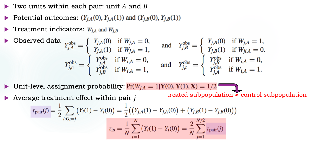
A special case of a SRE with J = N / 2 J=N/2 J = N /2
One treated and one control unit (a pair) within each stratum
Assignment probability:
P ( W ∣ X , Y ( 0 ) , Y ( 1 ) ) = ∏ j = 1 N / 2 1 2 = 2 − N / 2 for reasonable W , 0 for others P(\boldsymbol{W}\mid \boldsymbol{X},\boldsymbol{Y}(0),\boldsymbol{Y}(1))=\prod_{j=1}^{N/2} \frac{1}{2}=2^{-N/2}\ \text{for reasonable}\ \boldsymbol{W}, 0\ \text{for others}
P ( W ∣ X , Y ( 0 ) , Y ( 1 )) = j = 1 ∏ N /2 2 1 = 2 − N /2 for reasonable W , 0 for others
Intuition behind PREs
Within-pair variation in potential outcomes is less than between-pair variation -- gain in precision
If the population is relatively large, it may be possible to get very close matches of units in each pair
Notations
Causal Estimands in PREs
τ p a i r ( j ) = 1 2 ∑ i : G i = j ( Y i ( 1 ) − Y i ( 0 ) ) = 1 2 [ ( Y j , A ( 1 ) − Y j , A ( 0 ) ) + ( Y j , B ( 1 ) − Y j , B ( 0 ) ) ] \tau_{\mathrm{pair}}(j)=\frac{1}{2}\sum_{i:G_{i}=j} (Y_{i}(1)-Y_{i}(0))=\frac{1}{2}\left[ (Y_{j,A}(1)-Y_{j,A}(0))+ (Y_{j,B}(1)-Y_{j,B}(0)) \right]
τ pair ( j ) = 2 1 i : G i = j ∑ ( Y i ( 1 ) − Y i ( 0 )) = 2 1 [ ( Y j , A ( 1 ) − Y j , A ( 0 )) + ( Y j , B ( 1 ) − Y j , B ( 0 )) ]
τ f s = 1 N ∑ i = 1 N ( Y i ( 1 ) − Y i ( 0 ) ) = 2 N ∑ j = 1 N / 2 τ p a i r ( j ) \tau_{fs}=\frac{1}{N}\sum_{i=1}^{N} (Y_{i}(1)-Y_{i}(0))=\frac{2}{N}\sum_{j=1}^{N/2} \tau_{\mathrm{pair}}(j)
τ f s = N 1 i = 1 ∑ N ( Y i ( 1 ) − Y i ( 0 )) = N 2 j = 1 ∑ N /2 τ pair ( j )
Inference Approaches for PREs
Fisher's Exact P-Values
Same as SREs.
Neyman’s Repeated Sampling Approach
The Challenges
One treated and one control unit in each strata lead to specified challenges .
Let's see
τ ^ d i f = 2 N ∑ j = 1 N / 2 τ ^ p a i r ( j ) \hat{\tau}^{\mathrm{dif}}=\frac{2}{N}\sum_{j=1}^{N/2} \hat{\tau}_{\mathrm{pair}}(j)
τ ^ dif = N 2 j = 1 ∑ N /2 τ ^ pair ( j )
where τ ^ p a i r ( j ) = Y j , t o b s − Y j , c o b s = ∑ i : G i = j ( 2 W i − 1 ) Y i o b s \hat{\tau}^{\mathrm{pair}}(j)=Y^{\mathrm{obs}}_{j,t}-Y^{\mathrm{obs}}_{j,c}=\sum _{i:G_{i}=j}(2W_{i}-1)Y^{\mathrm{obs}}_{i} τ ^ pair ( j ) = Y j , t obs − Y j , c obs = ∑ i : G i = j ( 2 W i − 1 ) Y i obs
Can verify that
E W [ τ ^ p a i r ( j ) ] = τ f s ( j ) V W [ τ ^ p a i r ( j ) ] = S c ( j ) 2 N c ( j ) + S t ( j ) 2 N t ( j ) − S t c ( j ) 2 N ( j ) = S c ( j ) 2 + S t ( j ) 2 − S t c ( j ) 2 2 \begin{align}
\mathbb{E}_{W}[\hat{\tau}^{\mathrm{pair}}(j)] & =\tau_{fs}(j) \\
\mathbb{V}_{W}[\hat{\tau}^{\mathrm{pair}}(j)] & = \frac{S_{c}(j)^{2}}{N_{c}(j)}+\frac{S_{t}(j)^{2}}{N_{t}(j)}-\frac{S_{tc}(j)^{2}}{N(j)} \\
& = S_{c}(j)^{2}+S_{t}(j)^{2}-\frac{S_{tc}(j)^{2}}{2}
\end{align}
E W [ τ ^ pair ( j )] V W [ τ ^ pair ( j )] = τ f s ( j ) = N c ( j ) S c ( j ) 2 + N t ( j ) S t ( j ) 2 − N ( j ) S t c ( j ) 2 = S c ( j ) 2 + S t ( j ) 2 − 2 S t c ( j ) 2
So
E W [ τ ^ d i f ] = τ f s V W [ τ ^ d i f ] = ( 2 N ) 2 ⋅ ∑ j = 1 N / 2 ( S c ( j ) 2 + S t ( j ) 2 − S t c ( j ) 2 2 ) \begin{align}
\mathbb{E}_{W}[\hat{\tau}^{\mathrm{dif}}] & =\tau_{fs} \\
\mathbb{V}_{W}[\hat{\tau}^{\mathrm{dif}}] & = \left( \frac{2}{N} \right)^{2}\cdot\sum_{j=1}^{N/2} \left( S_{c}(j)^{2}+S_{t}(j)^{2}-\frac{S_{tc}(j)^{2}}{2} \right)
\end{align}
E W [ τ ^ dif ] V W [ τ ^ dif ] = τ f s = ( N 2 ) 2 ⋅ j = 1 ∑ N /2 ( S c ( j ) 2 + S t ( j ) 2 − 2 S t c ( j ) 2 )
Till now it seem good. Seems like we can use this to estimate and conduct inference. But we cannot estimate the finite sample variances S c ( j ) 2 , S t ( j ) 2 S_{c}(j)^{2}, S_{t}(j)^{2} S c ( j ) 2 , S t ( j ) 2 S t c ( j ) 2 S_{tc}(j)^{2} S t c ( j ) 2
constant treatment effect within pairs: Y j , A ( 1 ) − Y j , A ( 0 ) = Y j , B ( 1 ) − Y j , B ( 0 ) = : τ p a i r ( j ) ∀ j Y_{j,A}(1)-Y_{j,A}(0)=Y_{j,B}(1)-Y_{j,B}(0)=:\tau_{\mathrm{pair}}(j)\quad \forall j Y j , A ( 1 ) − Y j , A ( 0 ) = Y j , B ( 1 ) − Y j , B ( 0 ) =: τ pair ( j ) ∀ j
- This leads to $S_c^2(j)=S_t^2(j)=:S(j)$ and $S_{tc}^2(j)=0$. - So $\mathbb{V}_{W}[\hat{\tau}^{\mathrm{pair}}(j)]=2S^2(j)$. treatment effect is constant across pairs: τ p a i r ( j ) = τ f s ∀ j \tau_{\mathrm{pair}}(j)=\tau_{fs}\quad \forall j τ pair ( j ) = τ f s ∀ j
within-pair variances are constant: S 2 ( j ) = S 2 ∀ j S^{2}(j)=S^{2}\quad \forall j S 2 ( j ) = S 2 ∀ j
With this assumptions holding, we have
V W [ τ ^ d i f ] = ⋯ = 4 N S 2 \mathbb{V}_{W}[\hat{\tau}^{\mathrm{dif}}]=\dots=\frac{4}{N}S^{2}
V W [ τ ^ dif ] = ⋯ = N 4 S 2
A variance estimator can be proposed:
V ^ p a i r ( τ ^ d i f ) = 4 N ( N − 2 ) ∑ j = 1 N / 2 ( τ ^ p a i r ( j ) − τ ^ d i f ) 2 \hat{\mathbb{V}}^{\mathrm{pair}}(\hat{\tau}^{\mathrm{dif}})=\frac{4}{N(N-2)}\sum_{j=1}^{N/2} \left( \hat{\tau}^{\mathrm{pair}}(j)-\hat{\tau}^{\mathrm{dif}} \right)^{2}
V ^ pair ( τ ^ dif ) = N ( N − 2 ) 4 j = 1 ∑ N /2 ( τ ^ pair ( j ) − τ ^ dif ) 2
(Note that τ ^ d i f \hat{\tau}^{\mathrm{dif}} τ ^ dif τ ^ p a i r ( j ) \hat{\tau}^{\mathrm{pair}}(j) τ ^ pair ( j )
Assumption 1 and 2 are enough to keep the estimator unbiased.
Can show that
E [ V ^ p a i r ( τ ^ d i f ) ] = V W [ τ ^ d i f ] + 4 N ( N − 2 ) ∑ j = 1 N / 2 ( τ p a i r ( j ) − τ ) 2 \mathbb{E}[\hat{\mathbb{V}}^{\mathrm{pair}}(\hat{\tau}^{\mathrm{dif}})]=\mathbb{V}_{W}[\hat{\tau}^{\mathrm{dif}}]+\frac{4}{N(N-2)}\sum_{j=1}^{N/2}(\tau_{\mathrm{pair}}(j)-\tau)^{2}
E [ V ^ pair ( τ ^ dif )] = V W [ τ ^ dif ] + N ( N − 2 ) 4 j = 1 ∑ N /2 ( τ pair ( j ) − τ ) 2
Under the assumptions above, the estimator is unbiased. If there is heterogeneity in the treatment effects (i.e. τ p a i r ( j ) \tau_{\mathrm{pair}}(j) τ pair ( j ) upwardly biased , and the corresponding confidence intervals will be conservative but still valid .
▶
The math behind the variance estimator
We have N N N X 1 , … X N X_{1},\dots X_{N} X 1 , … X N μ \mu μ V [ X i ] = σ i 2 \mathbb{V}[X_{i}]=\sigma_{i}^{2} V [ X i ] = σ i 2
V [ X ˉ ] = 1 N 2 ∑ i = 1 N σ i 2 \mathbb{V}[\bar{X}]=\frac{1}{N^{2}}\sum_{i=1}^{N} \sigma_{i}^{2} V [ X ˉ ] = N 2 1 i = 1 ∑ N σ i 2
and it can be estimated by
s 2 N = 1 N ( N − 1 ) ∑ i = 1 N ( X i − X ˉ ) 2 \frac{s^{2}}{N}=\frac{1}{N(N-1)}\sum_{i=1}^{N} (X_{i}-\bar{X})^{2} N s 2 = N ( N − 1 ) 1 i = 1 ∑ N ( X i − X ˉ ) 2
because one can verify that
E [ s 2 N ] = 1 N 2 ∑ i = 1 N σ i 2 = V [ X ˉ ] \mathbb{E}\left[ \frac{s^{2}}{N} \right]=\frac{1}{N^{2}} \sum_{i=1}^{N} \sigma^{2}_{i}=\mathbb{V}[\bar{X}] E [ N s 2 ] = N 2 1 i = 1 ∑ N σ i 2 = V [ X ˉ ]
If the expectations are different, then
E [ s 2 N ] = V [ X ˉ ] + 1 N ( N − 1 ) ∑ i = 1 N ( μ i − μ ˉ ) 2 \mathbb{E}\left[ \frac{s^{2}}{N} \right]=\mathbb{V}[\bar{X}]+\frac{1}{N(N-1)}\sum_{i=1}^{N} (\mu_{i}-\bar{\mu})^{2} E [ N s 2 ] = V [ X ˉ ] + N ( N − 1 ) 1 i = 1 ∑ N ( μ i − μ ˉ ) 2
where μ i = E [ X i ] , μ ˉ = 1 N ∑ i = 1 N μ i \mu_{i}=\mathbb{E}[X_{i}],\bar{\mu}=\frac{1}{N}\sum_{i=1}^{N}\mu_{i} μ i = E [ X i ] , μ ˉ = N 1 ∑ i = 1 N μ i
∑ i = 1 N ( X i − μ ) 2 = ∑ i = 1 N ( X i − X ˉ ) 2 + ∑ i = 1 N ( X ˉ − μ ) 2 \sum_{i=1}^N(X_i-\mu)^2 = \sum_{i=1}^{N} (X_{i}-\bar{X})^{2}+\sum_{i=1}^{N} (\bar{X}-\mu)^{2} i = 1 ∑ N ( X i − μ ) 2 = i = 1 ∑ N ( X i − X ˉ ) 2 + i = 1 ∑ N ( X ˉ − μ ) 2
This is an algebraic identity (恒等式). The deviation of many numbers to a certain constant can be divided into two parts: the deviation from the mean and the deviation of the mean from the constant.
Regression Method
Four models are proposed:
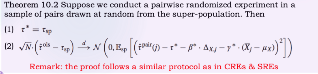
τ ^ p a i r ( j ) = τ + ε j \hat{\tau}^{\mathrm{pair}}(j)=\tau+\varepsilon_{j} τ ^ pair ( j ) = τ + ε j τ ^ p a i r ( j ) = τ + β Δ X , j + ε j \hat{\tau}^{\mathrm{pair}}(j)=\tau+\beta \Delta_{X,j}+\varepsilon_{j} τ ^ pair ( j ) = τ + β Δ X , j + ε j
Δ X , j = W j , A ( X j , A − X j , B ) + ( 1 − W j , A ) ( X j , B − X j , A ) \Delta_{X,j}=W_{j,A}(X_{j,A}-X_{j,B})+(1-W_{j,A})(X_{j,B}-X_{j,A})
Δ X , j = W j , A ( X j , A − X j , B ) + ( 1 − W j , A ) ( X j , B − X j , A )
alway ensure that it's the diff between treated one and controlled one.
τ ^ p a i r ( j ) = τ + γ ( X j ˉ − X ˉ ) + ε j \hat{\tau}^{\mathrm{pair}}(j)=\tau+\gamma(\bar{X_{j}}-\bar{X})+\varepsilon_{j} τ ^ pair ( j ) = τ + γ ( X j ˉ − X ˉ ) + ε j X ˉ j = ( X j , A + X j , B ) / 2 \bar{X}_{j}=(X_{j,A}+X_{j,B})/2 X ˉ j = ( X j , A + X j , B ) /2 τ ^ p a i r ( j ) = τ + β Δ X , j + γ ( X j ˉ − X ˉ ) + ε j \hat{\tau}^{\mathrm{pair}}(j)=\tau+\beta \Delta_{X,j}+\gamma(\bar{X_{j}}-\bar{X})+\varepsilon_{j} τ ^ pair ( j ) = τ + β Δ X , j + γ ( X j ˉ − X ˉ ) + ε j
For model 4, we have
大班教学还是小班教学
SUTVA,以班级为 unit 分层随机化,为了避免 Simpson's 悖论,相对 CRE 锦上添花,功效更高 FEP
每一层 τ ^ d i f \hat{\tau}^{\mathrm{dif}} τ ^ dif 加权平均 SRE 中,Y ˉ t o b s − Y ˉ c o b s \bar{Y}^{obs}_{t}-\bar{Y}^{obs}_{c} Y ˉ t o b s − Y ˉ c o b s H 0 H_{0} H 0 为啥秩统计量在 SRE 中不好? Neyman
τ ^ S R E \hat{\tau}^{SRE} τ ^ S R E SRE 满足无混杂假设,避免 Simpson's paradox,也就是 confoundedness bias 分层使得估计量方差更小 小多少,取决于 X X X P C R E ( W → = w → ∣ N → ) = P S R E ( W → = w → ) P_{CRE}(\overrightarrow{W}=\overrightarrow{w}\mid \overrightarrow{N})=P_{SRE}(\overrightarrow{W}=\overrightarrow{w}) P C R E ( W = w ∣ N ) = P S R E ( W = w ) 明明是 CRE 拿来的数据,可以当作 SRE 来分析 Post-stratification in a CRE 不要求每一组 ATE 一样 Reg
PRE
特殊的 SRE 改进精度,小方差 每层样本量只有 2 四种方法 FEP 不受影响 Model based 不受影响 Neyman 和 Reg 受样本量影响 每一对当成一个样本,作为 τ \tau τ τ \tau τ 回归 系数跟样本量一样多,过拟合,方差大,精度差 四种方法