Linear Regression with No Covariates
Recall that
Y i o b s = Y i ( 1 ) W i + Y i ( 0 ) ( 1 − W i ) , W i ⊥ ( Y i ( 1 ) , Y i ( 0 ) ) Y_{i}^{obs}=Y_{i}(1)W_i+Y_{i}(0)(1-W_{i}), \quad W_{i}\perp(Y_i(1),Y_i(0))
Y i o b s = Y i ( 1 ) W i + Y i ( 0 ) ( 1 − W i ) , W i ⊥ ( Y i ( 1 ) , Y i ( 0 ))
rearrange the terms:
Y i o b s = [ Y i ( 1 ) − Y i ( 0 ) ] W i + Y i ( 0 ) Y_{i}^{obs}=\left[ Y_{i}(1)-Y_{i}(0) \right] W_i + Y_{i}(0)
Y i o b s = [ Y i ( 1 ) − Y i ( 0 ) ] W i + Y i ( 0 )
I want to turn this into a linear regression model Y i o b s ∼ W i Y_{i}^{obs}\sim W_{i} Y i o b s ∼ W i
C o v ( Y i o b s , W i ) V a r ( W i ) = E [ [ Y i ( 1 ) − Y i ( 0 ) ] W i 2 ] − E [ [ Y i ( 1 ) − Y i ( 0 ) ] W i ] E [ W i ] E [ W i 2 ] − E [ W i ] 2 = … = τ s p \begin{align}
\frac{\mathrm{Cov}(Y_i^{obs},W_{i})}{\mathrm{Var}(W_i)} & = \frac{\mathbb{E}\left[ [ Y_{i}(1)-Y_{i}(0) ]W_{i}^{2} \right]-\mathbb{E} [[ Y_{i}(1)-Y_{i}(0) ]W_{i}]\mathbb{E}[W_i]}{\mathbb{E}[W_i^{2}]-\mathbb{E}[W_i]^{2}} \\
& = \dots \\
& = \tau_{sp}
\end{align}
Var ( W i ) Cov ( Y i o b s , W i ) = E [ W i 2 ] − E [ W i ] 2 E [ [ Y i ( 1 ) − Y i ( 0 )] W i 2 ] − E [[ Y i ( 1 ) − Y i ( 0 )] W i ] E [ W i ] = … = τ s p
The intercept is
E [ Y i o b s ] − τ s p E [ W i ] = ⋯ = μ c \mathbb{E}[Y_{i}^{obs}]-\tau_{sp}\mathbb{E}[W_i]=\dots=\mu_{c}
E [ Y i o b s ] − τ s p E [ W i ] = ⋯ = μ c
Therefore the following linear model can be set:
Y i o b s = α + τ W i + ε i Y_{i}^{obs}=\alpha+\tau W_i+\varepsilon_i
Y i o b s = α + τ W i + ε i
where α = μ c , τ = τ s p \alpha=\mu _{c},\ \tau=\tau _{sp} α = μ c , τ = τ s p
We can show that
ε i = { Y i ( 0 ) − μ c if W i = 0 Y i ( 1 ) − μ t if W i = 1 \varepsilon_i=\begin{cases}
Y_{i}(0)-\mu _{c} & \text{if}\ W_i=0 \\
Y_{i}(1)-\mu _{t} & \text{if}\ W_i=1
\end{cases}
ε i = { Y i ( 0 ) − μ c Y i ( 1 ) − μ t if W i = 0 if W i = 1
The OLS estimators α ^ , τ ^ \hat{\alpha},\hat{\tau} α ^ , τ ^ Y ˉ c o b s , Y ˉ t o b s − Y ˉ c o b s \bar{Y}_c^{obs}, \bar{Y}^{obs}_t-\bar{Y}^{obs}_c Y ˉ c o b s , Y ˉ t o b s − Y ˉ c o b s
Justification for Linear Regression
We'll see whether ε i \varepsilon _{i} ε i
Independence : Given all W i W_i W i ε i \varepsilon_i ε i ( Y i ( 1 ) , Y i ( 0 ) ) (Y_{i}(1),Y_{i}(0)) ( Y i ( 1 ) , Y i ( 0 )) ( Y i ( 1 ) , Y i ( 0 ) ) (Y_{i}(1),Y_{i}(0)) ( Y i ( 1 ) , Y i ( 0 )) ε i \varepsilon_i ε i here .Zero conditional mean : E [ ε i ∣ W i ] = 0 \mathbb{E}[\varepsilon _{i}\mid W_{i}]=0 E [ ε i ∣ W i ] = 0 W i ⊥ ( Y i ( 1 ) , Y i ( 0 ) ) W_i\perp(Y_{i}(1),Y_{i}(0)) W i ⊥ ( Y i ( 1 ) , Y i ( 0 )) Equal variances : V [ ε i ∣ W i ] = σ t 2 W i + σ c 2 ( 1 − W i ) \mathbb{V}[\varepsilon _{i}\mid W_{i}]=\sigma^{2}_{t}W_i+\sigma^{2}_{c}(1-W_i) V [ ε i ∣ W i ] = σ t 2 W i + σ c 2 ( 1 − W i ) σ t 2 = σ c 2 \sigma^{2}_{t}=\sigma^{2}_{c} σ t 2 = σ c 2 Exogenous : C o v ( W i , ε i ) = E [ W i ε i ] = 0 \mathrm{Cov}(W_{i},\varepsilon _{i})=\mathbb{E}[W_i\varepsilon_i]=0 Cov ( W i , ε i ) = E [ W i ε i ] = 0
Inference
Assume Equal Variances
Assume σ t = σ c = σ \sigma_{t}=\sigma_{c}=\sigma σ t = σ c = σ
Let
X = ( 1 N c 0 N c 1 N t 1 N t ) β = ( α τ ) X=\begin{pmatrix}
1_{N_c} & 0_{N_c} \\
1_{N_t} & 1_{N_t}
\end{pmatrix}\quad
\beta=\begin{pmatrix}
\alpha \\
\tau
\end{pmatrix}
X = ( 1 N c 1 N t 0 N c 1 N t ) β = ( α τ )
Then
Y o b s = X β + ε Y^{obs}=X\beta+\varepsilon
Y o b s = X β + ε
From Lec3-Statistical-Inference-and-Power we know
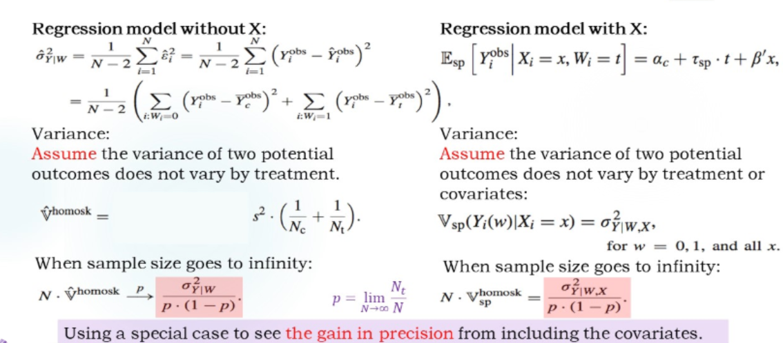
V [ τ ^ ] = σ 2 ∑ i = 1 N ( W i − W ˉ ) 2 = σ 2 ( 1 N c + 1 N t ) \mathbb{V}[\hat{\tau}]=\frac{\sigma^{2}}{\sum_{i=1}^{N} (W_{i}-\bar{W})^{2}}=\sigma^{2}\left( \frac{1}{N_c}+\frac{1}{N_t} \right)
V [ τ ^ ] = ∑ i = 1 N ( W i − W ˉ ) 2 σ 2 = σ 2 ( N c 1 + N t 1 )
And σ ^ 2 = s 2 = S S E N − 2 = 1 N − 2 ( s c 2 ( N c − 1 ) + s t 2 ( N t − 1 ) ) \hat{\sigma}^{2}=s^{2}=\frac{SSE}{N-2}=\frac{1}{N-2}\left( s_c^{2}(N_c-1)+s_t^{2}(N_t-1) \right) σ ^ 2 = s 2 = N − 2 S S E = N − 2 1 ( s c 2 ( N c − 1 ) + s t 2 ( N t − 1 ) ) V [ τ ^ ] \mathbb{V}[\hat{\tau}] V [ τ ^ ] V ^ c o n s t \hat{\mathbb{V}}^{\mathrm{const}} V ^ const here .
Allow Non-Equal Variances
The the robust variance estimator in linear regression is the same as V ^ n e y m a n = s c 2 N c + s t 2 N t \hat{\mathbb{V}}^{\mathrm{neyman}}=\frac{s^{2}_{c}}{N_{c}}+\frac{s^{2}_{t}}{N_{t}} V ^ neyman = N c s c 2 + N t s t 2
▶
The Hetero-Skedasticity-Robust Varicance Estimate
The model
Y = X β + ε Y=X\beta+\varepsilon Y = X β + ε
where each component of ε \varepsilon ε σ i 2 \sigma^{2}_{i} σ i 2
The estimator
β ^ = ( X T X ) − 1 X T Y = ( X T X ) − 1 X T ( X β + ε ) = β + ( X T X ) − 1 X T ε \hat{\beta}=(X^TX)^{-1}X^TY=(X^TX)^{-1}X^T(X\beta+\varepsilon)=\beta+(X^TX)^{-1}X^T\varepsilon β ^ = ( X T X ) − 1 X T Y = ( X T X ) − 1 X T ( X β + ε ) = β + ( X T X ) − 1 X T ε
The covariance matrix of β ^ \hat{\beta} β ^
V [ β ^ ] = ( X T X ) − 1 X T Σ X ( X T X ) − 1 \mathbb{V}[\hat{\beta}]=(X^TX)^{-1}X^T\Sigma X(X^TX)^{-1} V [ β ^ ] = ( X T X ) − 1 X T Σ X ( X T X ) − 1
where
Σ = d i a g ( σ i 2 ) \Sigma=\mathrm{diag}(\sigma^{2}_{i}) Σ = diag ( σ i 2 )
(Assume no correlation)
Σ ^ = d i a g ( e i 2 ) \hat{\Sigma}=\mathrm{diag}(e_{i}^{2}) Σ ^ = diag ( e i 2 )
can be used to estimate Σ \Sigma Σ
V ^ r o b u s t , H C 0 [ τ ^ ] = ∑ ( W i − W ˉ ) 2 e i 2 [ ∑ ( W i − W ˉ ) 2 ] 2 = … = ( N c 2 ( N t − 1 ) N 2 s t 2 + N t 2 ( N c − 1 ) N 2 s c 2 ) N 2 N c 2 N t 2 = ( N t − 1 ) s t 2 N t 2 + ( N c − 1 ) s c 2 N c 2 \begin{align}
\hat{\mathbb{V}}^{\mathrm{robust},HC_{0}}[\hat{\tau}] & = \frac{\sum (W_i-\bar{W})^{2}e_{i}^{2}}{\left[ \sum(W_i-\bar{W})^{2} \right]^{2}} \\
& = \dots \\
& = \left( \frac{N_c^{2}(N_{t}-1)}{N^{2}}s_t^{2}+\frac{N_t^{2}(N_c-1)}{N^{2}}s_c^{2} \right) \frac{N^{2}}{N_c^{2}N_t^{2}} \\
& = \frac{(N_{t}-1)s_t^{2}}{N_t^{2}}+\frac{(N_{c}-1)s_c^{2}}{N_c^{2}}
\end{align}
V ^ robust , H C 0 [ τ ^ ] = [ ∑ ( W i − W ˉ ) 2 ] 2 ∑ ( W i − W ˉ ) 2 e i 2 = … = ( N 2 N c 2 ( N t − 1 ) s t 2 + N 2 N t 2 ( N c − 1 ) s c 2 ) N c 2 N t 2 N 2 = N t 2 ( N t − 1 ) s t 2 + N c 2 ( N c − 1 ) s c 2
with HC2 adjustment,
V ^ r o b u s t , H C 2 [ τ ^ d i f ] = V ^ n e y m a n \hat{\mathbb{V}}^{\mathrm{robust},HC_{2}}[\hat{\tau}^{\mathrm{dif}}] = \hat{\mathbb{V}}^{\mathrm{neyman}}
V ^ robust , H C 2 [ τ ^ dif ] = V ^ neyman
Another Interpretation: Under Imputation (填补)
Recall the key challenge: missing data. So we cannot know each unit's treatment effect τ i \tau_{i} τ i
τ ^ i = { Y i ( 1 ) − Y ^ i ( 0 ) if W i = 1 Y ^ i ( 1 ) − Y i ( 0 ) if W i = 0 \hat{\tau}_i = \begin{cases}
Y_{i}(1)-\hat{Y}_{i}(0) & \text{if}\ W_i=1 \\
\hat Y_{i}(1)-Y_{i}(0) & \text{if}\ W_i=0 \\
\end{cases}
τ ^ i = { Y i ( 1 ) − Y ^ i ( 0 ) Y ^ i ( 1 ) − Y i ( 0 ) if W i = 1 if W i = 0
where Y ^ i ( 0 ) = Y ˉ c o b s , Y ^ i ( 1 ) = Y ˉ t o b s \hat{Y}_{i}(0)=\bar Y^{obs}_c, \hat{Y}_i(1)=\bar{Y}^{obs}_{t} Y ^ i ( 0 ) = Y ˉ c o b s , Y ^ i ( 1 ) = Y ˉ t o b s
Then use τ ^ = 1 N ∑ i = 1 N τ ^ i \hat{\tau}=\frac{1}{N}\sum_{i=1}^{N}\hat{\tau}_{i} τ ^ = N 1 ∑ i = 1 N τ ^ i τ s p \tau_{sp} τ s p Y ˉ t o b s − Y ˉ c o b s \bar{Y}^{obs}_{t}-\bar{Y}^{obs}_{c} Y ˉ t o b s − Y ˉ c o b s
Yet Another Interpretation: Under Limitation
The regression model is
Y i o b s = α + τ W i + ε i Y_{i}^{obs}=\alpha+\tau W_{i}+\varepsilon_{i}
Y i o b s = α + τ W i + ε i
LS estimate
( τ ^ , α ^ ) = argmin α , τ ∑ i = 1 N ( Y i o b s − α − τ W i ) 2 = argmin α , τ 1 N ∑ i = 1 N ( Y i o b s − α − τ W i ) 2 (\hat{\tau},\hat{\alpha})=\operatorname*{argmin}_{\alpha,\tau}\sum_{i=1}^{N} (Y^{obs}_{i}-\alpha-\tau W_{i})^{2}=\operatorname*{argmin}_{\alpha,\tau}{\color{blue}\frac{1}{N}}\sum_{i=1}^{N} (Y^{obs}_{i}-\alpha-\tau W_{i})^{2}
( τ ^ , α ^ ) = α , τ argmin i = 1 ∑ N ( Y i o b s − α − τ W i ) 2 = α , τ argmin N 1 i = 1 ∑ N ( Y i o b s − α − τ W i ) 2
When sample size goes to infinity
( α ∗ , τ ∗ ) = argmin α , τ E [ ( Y i o b s − α − τ W i ) 2 ] (\alpha^*,\tau^{*})=\operatorname*{argmin}_{\alpha,\tau}\mathbb{E}\left[ (Y^{obs}_{i}-\alpha-\tau W_{i})^{2} \right]
( α ∗ , τ ∗ ) = α , τ argmin E [ ( Y i o b s − α − τ W i ) 2 ]
We know from the OLS theory E [ Y i o b s ∣ W i ] = α ∗ + τ ∗ W i \mathbb{E}[Y_{i}^{obs}\mid W_{i}]=\alpha^{*}+\tau^{*}W_i E [ Y i o b s ∣ W i ] = α ∗ + τ ∗ W i
τ ∗ = E [ Y i o b s ∣ W i = 1 ] − E [ Y i o b s ∣ W i = 0 ] \tau^{*}=\mathbb{E}[Y_{i}^{obs}\mid W_{i}=1]-\mathbb{E}[Y_{i}^{obs}\mid W_{i}=0]
τ ∗ = E [ Y i o b s ∣ W i = 1 ] − E [ Y i o b s ∣ W i = 0 ]
With CRE,
τ ∗ = E [ Y i o b s ∣ W i = 1 ] − E [ Y i o b s ∣ W i = 0 ] = E [ Y i ( 1 ) ∣ W i = 1 ] − E [ Y i ( 0 ) ∣ W i = 0 ] = E [ Y i ( 1 ) ] − E [ Y i ( 0 ) ] = τ s p \begin{align}
\tau^{*} & = \mathbb{E}[Y_{i}^{obs}\mid W_{i}=1]-\mathbb{E}[Y_{i}^{obs}\mid W_{i}=0] \\
& = \mathbb{E}[Y_{i}(1)\mid W_{i}=1]-\mathbb{E}[Y_{i}(0)\mid W_{i}=0] \\
& = \mathbb{E}[Y_{i}(1)]-\mathbb{E}[Y_{i}(0)] \\
& = \tau_{sp}
\end{align}
τ ∗ = E [ Y i o b s ∣ W i = 1 ] − E [ Y i o b s ∣ W i = 0 ] = E [ Y i ( 1 ) ∣ W i = 1 ] − E [ Y i ( 0 ) ∣ W i = 0 ] = E [ Y i ( 1 )] − E [ Y i ( 0 )] = τ s p
Here is a more elementary proof.
Note that τ ^ → p τ ∗ \hat{\tau}\overset{p}{\to}\tau^* τ ^ → p τ ∗
Linear Regression with Covariates
Add Covariates
Regression model:
Y i o b s = α + τ W i + X i β + ε i Y_{i}^{obs}=\alpha+\tau W_{i} + X_{i}\beta+\varepsilon_{i}
Y i o b s = α + τ W i + X i β + ε i
where X i X_{i} X i
Similarly, when sample size goes to infinity
( τ ^ o l s , α ^ o l s , β ^ o l s ) → ( τ ∗ , α ∗ , β ∗ ) (\hat{\tau}^{ols},\hat{\alpha}^{ol s},\hat{\beta}^{ol s})\to (\tau^{*},\alpha^{*},\beta^{*})
( τ ^ o l s , α ^ o l s , β ^ o l s ) → ( τ ∗ , α ∗ , β ∗ )
where ( τ ∗ , α ∗ , β ∗ ) (\tau^{*},\alpha^{*},\beta^{*}) ( τ ∗ , α ∗ , β ∗ )
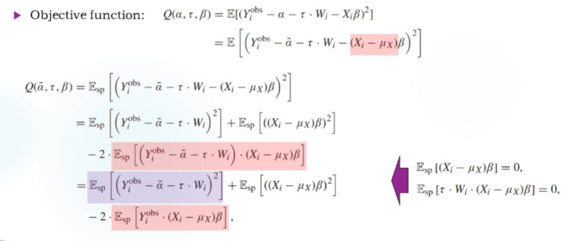
( τ ∗ , α ∗ , β ∗ ) = argmin α , β , τ E [ ( Y i o b s − α − τ W i − X i β ) 2 ] (\tau^{*},\alpha^{*},\beta^{*})=\operatorname*{argmin}_{\alpha,\beta,\tau}\mathbb{E}[(Y_{i}^{obs}-\alpha-\tau W_{i}-X_{i}\beta)^{2}]
( τ ∗ , α ∗ , β ∗ ) = α , β , τ argmin E [( Y i o b s − α − τ W i − X i β ) 2 ]
Okay, lets see E [ … ] \mathbb{E}[\dots] E [ … ]
We can deal with ( α ~ , τ ) (\tilde{\alpha},\tau) ( α ~ , τ ) β \beta β conclusion before, we know that τ ∗ = τ s p \tau^{*}=\tau_{sp} τ ∗ = τ s p
Theorem: Suppose we conduct a completely randomized experiment in a sample drawn at random from an infinite population. Then
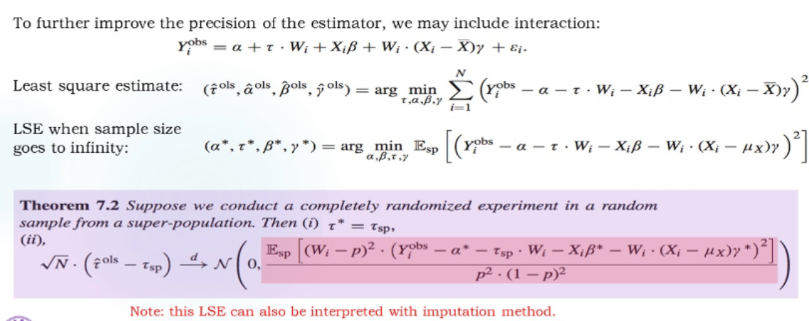
( 1 ) τ ∗ = τ s p ( 2 ) N ( τ ^ o l s − τ s p ) → d N ( 0 , E [ ( W i − p ) 2 ( Y i o l s − α ∗ − τ s p W i − X i β ∗ ) 2 ] p 2 ( 1 − p ) 2 ) \begin{aligned} (1)\ &\tau^{*}=\tau_{sp}\\ (2)\ &\sqrt{N}(\hat{\tau}^{ol s}-\tau_{sp})\overset{d}{\to}N\left( 0, \frac{\mathbb{E}\left[ (W_{i}-p)^{2}(Y_{i}^{ol s}-\alpha^{*}-\tau_{sp}W_{i}-X_{i}\beta^{*})^{2} \right] }{p^{2}(1-p)^{2}} \right) \end{aligned} ( 1 ) ( 2 ) τ ∗ = τ s p N ( τ ^ o l s − τ s p ) → d N ( 0 , p 2 ( 1 − p ) 2 E [ ( W i − p ) 2 ( Y i o l s − α ∗ − τ s p W i − X i β ∗ ) 2 ] )
where p = E [ W i ] p=\mathbb{E}[W_{i}] p = E [ W i ]
Connect the variance's shape with the sandwich variance estimator introduced above. The theorem is still correct even if the regression model is wrong.
Model Comparisons
Adding covariates can reduce the variance of τ ^ o l s \hat{\tau}^{ol s} τ ^ o l s
Add Interaction Term
Why adding interaction term? Because Y ( 1 ) ∼ X Y(1)\sim X Y ( 1 ) ∼ X Y ( 0 ) ∼ X Y(0)\sim X Y ( 0 ) ∼ X X X X
This perspective has not been introduced until 2008. But Fisher already added covariates into the regression model. Why he didn't notice this? The potential outcome framework was not invented by then. Without a good expression, people cannot see through things well.
GPT's summary:
正确识别加入协变量的回归式
回归 非参 线性模型错的,仍然可用
加入协变量,减小方差。-> 协变量越多越好?并非,虽然理论上放进来不会更差,但有限样本,分得越细,样本越少,估计越不准。
有时引入协变量方差会变大。 Y ( 1 ) , Y ( 0 ) Y(1),Y(0) Y ( 1 ) , Y ( 0 ) X X X X W XW X W
Fisher 早就提出加入协变量回归,但一直没发现问题。语言不好,框架不好(彼时没有潜在结果的语言)
机器学习的估计很难给出区间估计,不知其渐进分布。