线性回归分析-HW3

原题.

Prob-1

$$\begin{align} b_1 & = \frac{S_{xy}}{S_{xx}} \\ & =\beta_1 + \sum \frac{X_i-\bar{X}}{S_{xx}}\varepsilon_i \\ & \Downarrow \\ \mathbb{E}[b_{1}] & = \beta_{1} \end{align}$$

---

$$\begin{align} b_0 & = \bar{y}-b_1\bar{x} \\ & = \beta_0+\beta_{1}\bar{x}+\bar{\varepsilon}-b_{1}\bar{x} \\ & \Downarrow \\ \mathbb{E}[b_{0}] & = \beta_{0} \end{align}$$

---

$$\begin{align} \mathbb{E}[SSE] & = \mathbb{E}\left[ \sum_{i=1}^{N} e_i^{2} \right] \\ & = \mathbb{E}\left[ \sum_{i=1}^{N}\left[y_i-\left( \bar{y}-\frac{S_{xy}}{S_{xx}}\bar{x}+\frac{S_{xy}}{S_{xx}}x_{i} \right) \right]^{2} \right] \\ & = \mathbb{E}\left[ \sum_{i=1}^{N} \left( y_i-\bar{y}-\frac{S_{xy}}{S_{xx}}(x_i-\bar{x}) \right)^{2} \right] \\ & = \mathbb{E}[S_{yy}-\hat{\beta}_1^{2}S_{xx}] \end{align}$$

Since

$$S_{yy}=\beta_1^{2}S_{xx}+\sum_{i=1}^{N} (\varepsilon_i-\bar{\varepsilon})^{2}+2\sum_{i=1}^{N} \beta_{1}(x_i-\bar{x})(\varepsilon_i-\bar{\varepsilon}),$$

we have

$$\mathbb{E}[S_{yy}]=\beta_{1}^{2}S_{xx}+(n-1)\sigma^{2}$$

And

$$\mathbb{E}[\hat{\beta}_1^{2}S_{xx}]=S_{xx}\mathbb{E}[\hat{\beta}_1^{2}]=S_{xx}\left( \frac{\sigma^{2}}{S_{xx}}+\beta_{1}^{2} \right)$$

So

$$\mathbb{E}[SSE]=(n-2)\sigma^{2}$$

Prob-2

Let $b_{0}=\sum a_{i}Y_{i}$, where $a_{i}=\frac{1}{N}+\frac{\bar{X}(X_{i}-\bar{X})}{S_{xx}}$

Take any other linear estimator of $\beta_{0}$:

$$\tilde\beta_0 = \sum w_i Y_i, \qquad w_i = a_i + d_i,$$

Unbiasedness requires

$$\sum d_i = 0, \qquad \sum d_i X_i = 0.$$

which leads to $\sum a_{i}d_{i}=0$

Let's see the variance:

$$\mathbb{V}[\tilde{\beta}_{0}]=\sigma^{2}\sum (a_{i}+d_{i})^{2}=\sigma^{2}\left( \sum a_{i}^{2}+\sum d_{i}^{2} \right) \geq \sigma^{2}\sum a_{i}^{2}=\mathbb{V}[b_0]$$

The equality holds iff $d_{i}=0\ \forall i$.

So $b_{0}$ is the best among them.

Prob-3

a.

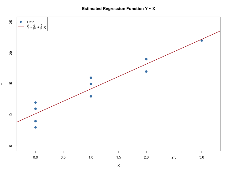
The estimated regression function is

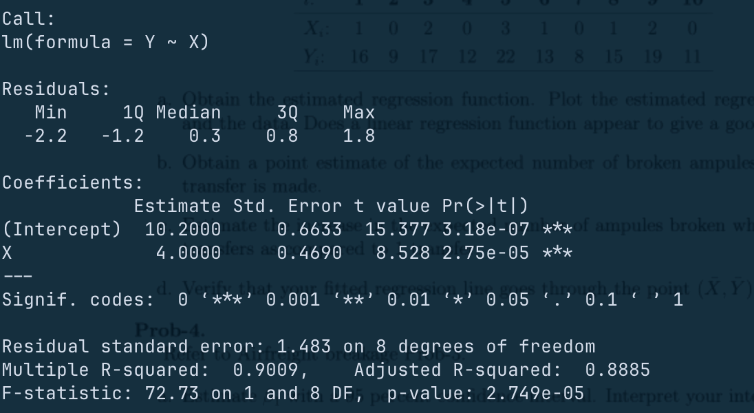
$$\hat{y}=10.2+4x$$

It appears good.

b.

14.2

c.

4

d.

$$\bar{X}=1\quad \bar{Y}=14.2$$

$$14.2=\bar{Y}=10.2 + 4\bar{X}=10.2+4$$

Prob-4

a.

95% CI

$$[b_{1}\pm t_{0.975,8}\cdot s(b_{1})]=[2.918, 5.082]$$

Interpretation:

Keep sampling and calculate the CI, 95% of the CIs cover the real value.

b.

$$\begin{align} H_{0} & : \beta_{1}=0 \\ H_{a} & : \beta_{1} \ne 0 \end{align}$$

Test statistic:

$$t=\frac{b_{1}}{s(b_{1})}=4.0 / 0.469 = 8.53$$

Decision rule:

$$\text{reject if}\ |t|>t_{0.975,8}=2.306$$

Conclusion: there is a linear association.

P value is $0.0000275$.

c.

95% CI

$$[b_{0}\pm t_{0.975,8}s(b_{0})]= [8.670, 11.730]$$

Interpretation:

Keep sampling and calculate the CI, 95% of the CIs cover the real value.

d.

Alternatives

$$\begin{align} H_{0} & : \beta_{0}\leq 9 \\ H_{a} & : \beta_{0} > 9 \end{align}$$

Test statistic

$$t=\frac{b_{0}-9}{s(b_{0})}=1.809$$

Decision rule: reject if $t>t_{0.975,8}=2.306$

Conclusion: At the 0.025 significance level there is not sufficient evidence that the mean number of broken ampules with no transfers exceeds 9.0.

P-value: 0.054

e.

If $\beta_{1}=2.0$,

$$\frac{b_{1}}{s(b_{1})}\sim t\left( 8, \frac{2}{.5} \right)$$

the power is

$$P\left( \frac{|b_{1}|}{s(b_{1})}>2.306 \right)=0.9367$$

If $\beta_{0}=11$,

$$\frac{b_{0}-9}{s(b_{0})}\sim t\left( 8, \frac{11-9}{.75} \right)$$

the power is

$$P\left( \frac{b_0}{s(b_{0})}>2.306 \right)=0.648$$