5 Assignment Design

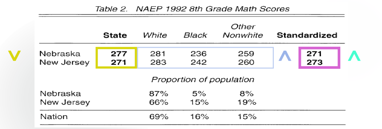
Intro -- Simpson's Paradox

The overall order is reversed after looking at each group. If the question is that, if a child is to be sent to one of the states to receive education, which one would be a better choice, then the overall index cannot be trusted.

The reason why this paradox happens is that the distribution of the covariate XX, which is the unit's race, is different between the two groups. This is equivalent to the difference in assignment mechanism WW across each race group. The following example explains:

group1 group2
Treat aa bb
Control cc dd

ab=cd  ⟺  ac=bd\frac{a}{b}=\frac{c}{d}\iff \frac{a}{c}=\frac{b}{d}

This is math from elementary school.

So we need to know the assignment mechanism before conducting correct inferences.

Note that even in CREs, Simpson's paradox can still happen. If it happens that the distribution of the covariate differs between the treated group and the control group, though it doesn't affect the validity of the estimator.

Definitions for Assignment Mechanism

Three Concepts

Definition (Assignment Mechanism)
Given a population of NN units, the assignment mechanism is a row-exchangeable function P(W∣X,Y(0),Y(1))P(\boldsymbol{W}\mid \boldsymbol{X},\boldsymbol{Y}(0),\boldsymbol{Y}(1)), taking on values in [0,1][0,1], satisfying

∑W∈{0,1}NP(W∣X,Y(0),Y(1))=1, ∀X,Y(0),Y(1)\sum _{W\in\{0,1\}^{N}} P(\boldsymbol{W}\mid \boldsymbol{X},\boldsymbol{Y}(0),\boldsymbol{Y}(1))=1,\ \forall \boldsymbol{X},\boldsymbol{Y}(0),\boldsymbol{Y}(1)

Definition (Unit Assignment Probability)

pi(X,Y(0),Y(1))=P(Wi=1∣X,Y(0),Y(1))p_{i}(\boldsymbol{X},\boldsymbol{Y}(0),\boldsymbol{Y}(1))=P(W_{i}=1\mid \boldsymbol{X},\boldsymbol{Y}(0),\boldsymbol{Y}(1))

Definition (Finite Population Propensity Score)
The propensity score at xx is the average unit assignment probability for units with Xi=xX_{i}=x,

e(x)=1N(x)∑i:Xi=xpi(X,Y(1),Y(0))e(x)=\frac{1}{N(x)}\sum _{i:X_{i}=x}p_{i}(\boldsymbol{X},\boldsymbol{Y}(1),\boldsymbol{Y}(0))

where N(x)=#{i∈{1,2,…,N}:Xi=x}N(x)=\#\{i\in\{1,2,\dots, N\}:X_{i}=x\} is the number of units with Xi=xX_{i}=x. If N(x)=0,e(x)N(x)=0, e(x) is defined to be 00.

Examples

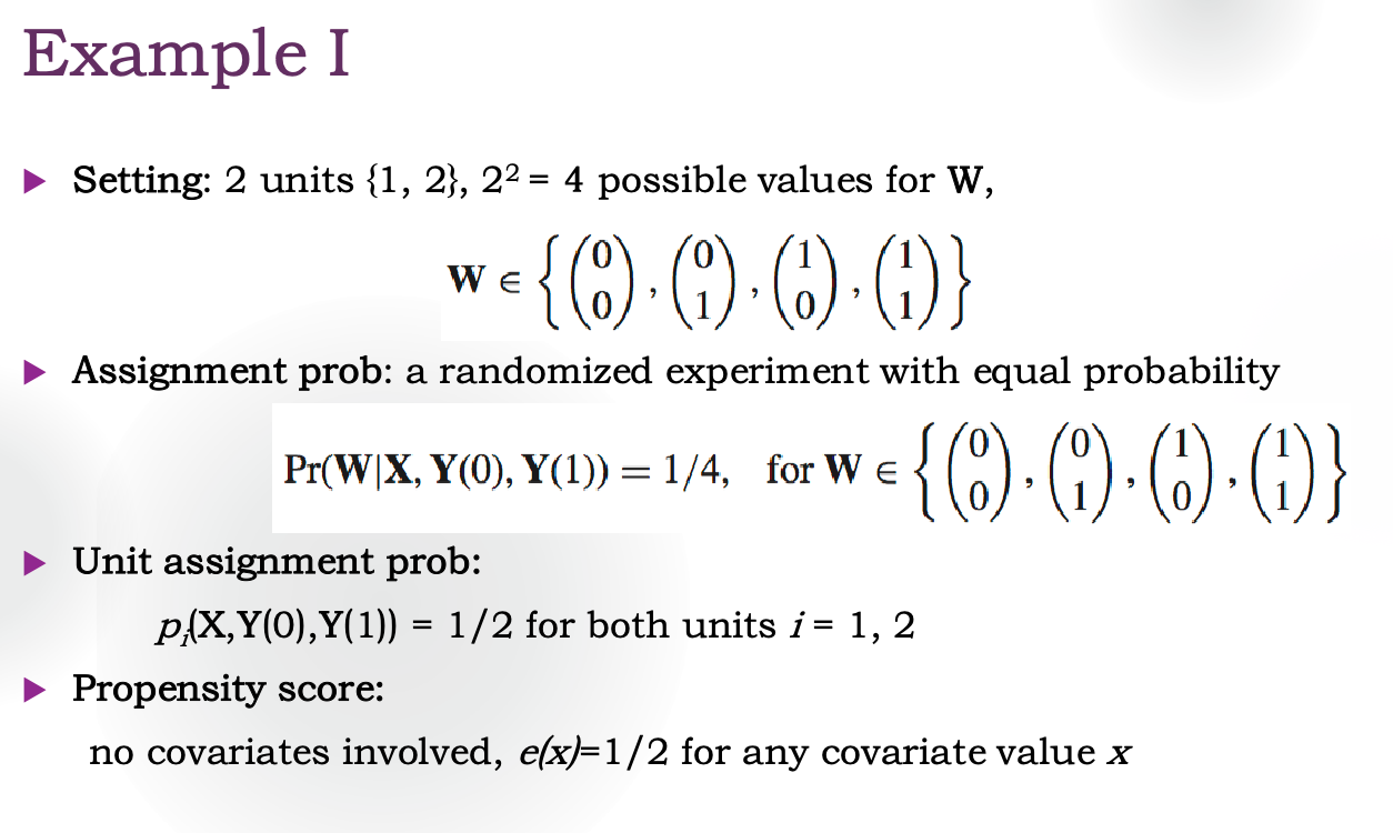
Bernoulli Randomization

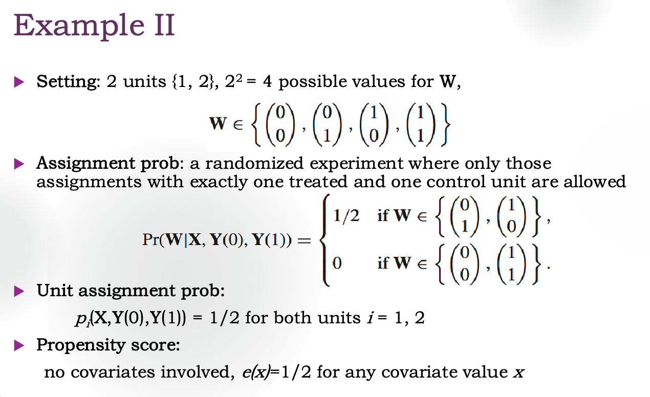
Complete Randomization

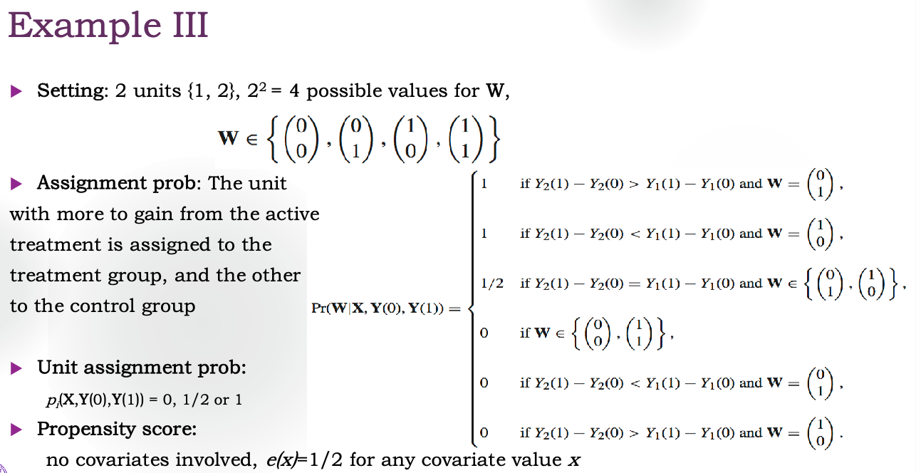
Some notes on example III:

Because there is no covariate, the propensity score degrades to

e(x)=1N∑i=1Npi(Y(1),Y(0))e(x)=\frac{1}{N}\sum_{i=1}^{N} p_{i}(\boldsymbol{Y}(1),\boldsymbol{Y}(0))

Whatever Y(1),Y(0)\boldsymbol{Y}(1),\boldsymbol{Y}(0) are, e(x)=12e(x)=\frac{1}{2}. It's easy to verify.


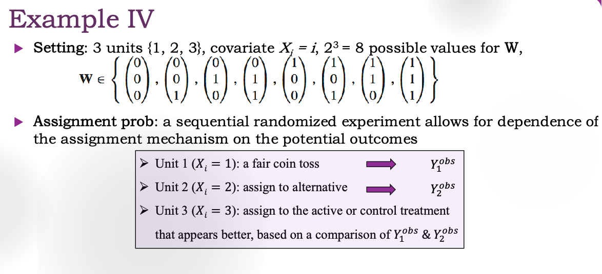
Below is a more complex example.

Suppose there always is a better one

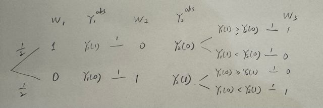
A sequential tree should be used to analyze this example.

Let A=Y1(1)−Y2(0),B=Y1(0)−Y2(1)A=Y_{1}(1)-Y_{2}(0), B=Y_{1}(0)-Y_{2}(1). Then the value space of Y(1),Y(0)\boldsymbol{Y}(1),\boldsymbol{Y}(0) can be divided into four mutually exclusive parts:

(1) A>0,B>0(2) A>0,B<0(3) A<0,B>0(4) A<0,B<0\begin{align} (1)\ & A>0,B>0 \\ (2)\ & A>0,B<0 \\ (3)\ & A<0,B>0 \\ (4)\ & A<0,B<0 \end{align}

For the first part, W\boldsymbol{W} can only be (1,0,1)(1,0,1) and (0,1,0)(0,1,0) with equal probs 0.50.5. Similarly we can get the full assignment mechanism.

As for the unit assignment prob., we can easily verify that

p1(X,Y(0),Y(1))=p2(X,Y(0),Y(1))=12p_{1}(\boldsymbol{X},\boldsymbol{Y}(0),\boldsymbol{Y}(1))=p_{2}(\boldsymbol{X},\boldsymbol{Y}(0),\boldsymbol{Y}(1))=\frac{1}{2}

(Note that it doesn't matter if we add X\boldsymbol{X} or not because the assignment mechanism, in this setting, has nothing to do with X\boldsymbol{X}.)

For the 3rd unit, we have

p3(X,Y(0),Y(1))={1/2,A>0, B>01,A>0, B<00,A<0, B>01/2,A<0, B<0p_{3}(\boldsymbol{X},\boldsymbol{Y}(0),\boldsymbol{Y}(1)) = \begin{cases} 1/2, & A>0,\ B>0 \\ 1, & A>0,\ B<0 \\ 0, & A<0,\ B>0 \\ 1/2, & A<0,\ B<0 \end{cases}

Let's talk about the (finite sample) propensity score now:

e(1)=p1(X,Y(0),Y(1))e(2)=p2(X,Y(0),Y(1))e(3)=p3(X,Y(0),Y(1))\begin{align} e(1) & =p_{1}(\boldsymbol{X},\boldsymbol{Y}(0),\boldsymbol{Y}(1)) \\ e(2) & =p_{2}(\boldsymbol{X},\boldsymbol{Y}(0),\boldsymbol{Y}(1)) \\ e(3) & = p_{3}(\boldsymbol{X},\boldsymbol{Y}(0),\boldsymbol{Y}(1)) \end{align}

世界运行规律(X,Y(0),Y(1)\boldsymbol{X},\boldsymbol{Y}(0),\boldsymbol{Y}(1))就那一套,但我们不知道是哪一套,所以分情况讨论

Assumptions for Assignment Mechanism

The four examples above are somewhat complex already though the number of the units is rather small. Cannot imagine how hard it would be if the number of units becomes large. So we need some assumptions to simplify our analysis.

Assumptions

Definition (Individualistic Assignment)
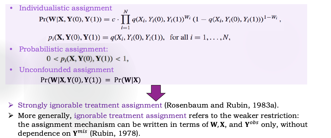
An assignment mechanism P(W∣X,Y(0),Y(1))P(\boldsymbol{W}\mid \boldsymbol{X},\boldsymbol{Y}(0),\boldsymbol{Y}(1)) is individualistic if, for some function q(⋅)∈[0,1]q(\cdot)\in [0,1],

pi(X,Y(0),Y(1))=q(Xi,Yi(0),Yi(1))∀i=1,…,Np_{i}(\boldsymbol{X},\boldsymbol{Y}(0),\boldsymbol{Y}(1))=q(X_{i},Y_{i}(0),Y_{i}(1))\quad\forall i=1,\dots,N

and

P(W∣X,Y(0),Y(1))=c⋅∏i=1Nq(Xi,Yi(0),Yi(1))Wi(1−q(Xi,Yi(0),Yi(1)))1−WiP(\boldsymbol{W}\mid \boldsymbol{X},\boldsymbol{Y}(0),\boldsymbol{Y}(1))=c\cdot \prod_{i=1}^{N} q(X_{i},Y_{i}(0),Y_{i}(1))^{W_{i}}(1-q(X_{i},Y_{i}(0),Y_{i}(1)))^{1-W_{i}}

for (W,X,Y(0),Y(1))∈A(\boldsymbol{W}, \boldsymbol{X},\boldsymbol{Y}(0),\boldsymbol{Y}(1))\in \mathbb{A}, for some set A\mathbb{A}, and 0 elsewhere (cc is the constant that ensures that the probabilities sum to unity).

The line ⋯∏…\dots\prod\dots is weaker than saying that WiW_{i}'s are independent given X,Y(0),Y(1)\boldsymbol{X},\boldsymbol{Y}(0),\boldsymbol{Y}(1). For example, complete randomization satisfies this.

Example IV above doesn't satisfy this.

Given individualistic assignment, the propensity score simplifies to

e(x)=1Nx∑i:Xi=xq(Xi,Yi(0),Yi(1))e(x)=\frac{1}{N_{x}}\sum _{i:X_{i}=x}q(X_{i},Y_{i}(0),Y_{i}(1))

3N3N-variate function →\to 3-variate function.


Definition (Probabilistic Assignment)
An assignment mechanism P(W∣X,Y(0),Y(1))P(\boldsymbol{W}\mid \boldsymbol{X},\boldsymbol{Y}(0),\boldsymbol{Y}(1)) is probabilistic if the probability of assignment to treatment for unit ii is strictly between zero and one:

pi(X,Y(0),Y(1))∈(0,1), for each possible X,Y(0),Y(1)p_{i}(\boldsymbol{X},\boldsymbol{Y}(0),\boldsymbol{Y}(1))\in (0,1),\ \text{for each possible}\ \boldsymbol{X},\boldsymbol{Y}(0),\boldsymbol{Y}(1)

for all i=1,…,Ni=1,\dots,N.

Don't know the purpose of this assumption.


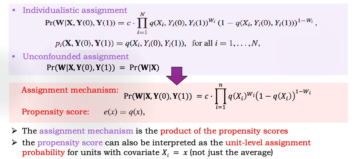
Definition (Unconfounded Assignment)
An assignment mechanism is unconfounded if it does not depend on the potential outcomes:

P(W∣X,Y(0),Y(1))=P(W∣X,Y′(0),Y′(1))P(\boldsymbol{W}\mid \boldsymbol{X},\boldsymbol{Y}(0),\boldsymbol{Y}(1))=P(\boldsymbol{W}\mid \boldsymbol{X},\boldsymbol{Y}'(0),\boldsymbol{Y}'(1))

for all W,X,Y(0),Y(1),Y′(0),Y′(1)\boldsymbol{W},\boldsymbol{X},\boldsymbol{Y}(0),\boldsymbol{Y}(1),\boldsymbol{Y}'(0),\boldsymbol{Y}'(1).

If an assignment mechanism is unconfounded, we can drop the two potential outcomes and write the assignment mechanism as P(W∣X)P(\boldsymbol{W}\mid \boldsymbol{X}).

This kind of assignment can avoid Simpson's paradox. Why?

Application

Here is an example of application, which will be used here. Suppose Xi∈{f,m}X_{i}\in \{f,m\}. Then

P(W∣X,Y(0),Y(1))=c⋅e(f)Nt(f)[1−e(f)]Nc(f)⋅e(m)Nt(m)[1−e(m)]Nc(m)P(\mathbf W\mid\mathbf X,\mathbf Y(0),\mathbf Y(1)) =c\cdot e(f)^{N_t(f)}[1-e(f)]^{N_c(f)}\cdot e(m)^{N_t(m)}[1-e(m)]^{N_c(m)}

for W∈A\boldsymbol{W}\in \mathbb{A}, where Nt(f)=∑i:Xi=fWi,Nc(f)=∑i:Xi=f(1−Wi)N_{t}(f)=\sum _{i:X_{i}=f}W_{i},N_{c}(f)=\sum _{i:X_{i}=f}(1-W_{i})...

So if we further condition on Nt(f)N_{t}(f) and Nt(m)N_{t}(m), then for W∈A,\boldsymbol{W}\in \mathbb{A}, the assignment probabilities are all the same. Therefore

P(W∣X,Y(0),Y(1),Nt(f),Nt(m))=1(N(f)Nt(f))(N(m)Nt(m))P(\mathbf W\mid\mathbf X,\mathbf Y(0),\mathbf Y(1),N_{t}(f),N_{t}(m))= \frac{1}{\binom{N(f)}{N_{t}(f)}\binom{N(m)}{N_t(m)}}

and one step forward, we have

P(Wi=1∣… )={1(N(f)Nt(f))(N(m)Nt(m))⋅(N(f)−1Nt(f)−1)⋅(N(m)Nt(m))=Nt(f)N(f)Xi=f1(N(f)Nt(f))(N(m)Nt(m))⋅(N(m)−1Nt(m)−1)⋅(N(f)Nt(f))=Nt(m)N(m)Xi=mP(W_{i}=1\mid \dots)= \begin{cases} \frac{1}{\binom{N(f)}{N_{t}(f)}\binom{N(m)}{N_t(m)}}\cdot \binom{N(f)-1}{N_{t}(f)-1}\cdot \binom{N(m)}{N_{t}(m)} = \frac{N_{t}(f)}{N(f)} & X_{i}=f\\ \frac{1}{\binom{N(f)}{N_{t}(f)}\binom{N(m)}{N_t(m)}}\cdot \binom{N(m)-1}{N_{t}(m)-1}\cdot \binom{N(f)}{N_{t}(f)}=\frac{N_{t}(m)}{N(m)} & X_{i}=m \end{cases}


  • Simpson's Paradox,权重,统计学常见现象
    • YY 跟 XX 有关
    • WW 跟 X,YX,Y 都有关,这种协变量称为混杂变量。confounding, confounding bias,会得出错误因果作用推断
    • 协变量分布平衡,即无矛盾
  • 分配机制 P(W∣Y(1),Y(0),X)P(\boldsymbol{W}\mid \boldsymbol{Y}(1),\boldsymbol{Y}(0),\boldsymbol{X}). 随机性来自有限总体那一层
    • 向量概率
    • 个体概率
    • 倾向得分(最重要)
  • 倾向得分,横着比例一样   ⟺  \iff 竖着比例一样
    • 为啥非得竖着看?倾向得分一样的可以打包起来一起算
  • 序贯树
  • 三个重要假设
    1. 个体化假设:降维,同一个函数
    2. 无混杂假设,条件独立(最根本,克服缺失数据问题,但没办法检验)
    3. 概率假设

5 Assignment Design
https://wtx17.github.io/2026/10/21/5-Assignment-Design/
作者
wtx
发布于
2026年10月21日
更新于
2026年11月6日
许可协议