概统拾遗

数据类型

截面数据

• 同一时间点或同一个时间段内，收集的多个个体的数据。
• 数据有“个体”维度，但没有“时间”维度。它反映的是不同个体在同一时刻的“快照”状态。

例子：某公司同一年度内，所有员工的年龄、工龄和薪资。

时间序列数据

• 对同一个个体（或同一个统计指标），在不同时间点上连续观测得到的数据
• 数据有“时间”维度，但没有“个体”维度（通常只有一个主体）。它反映的是该主体随时间变化的动态轨迹。

例子：某只股票一天内的每分钟价格。

面板数据

• 同时包含了截面数据和时间序列数据特征的二维数据。它是对多个个体，在多个时间点上进行的观测。
• 同时拥有“个体”和“时间”两个维度。既可以分析个体间的差异，也可以分析个体随时间变化的动态规律，还能研究两者的交互作用。

例子：在一项医学研究中，100名病人（个体）在手术后连续10周（时间）每周记录一次的健康指标。

三门问题

这个问题背景先不写了。

这问题为啥著名，因为它难，难搞清楚，就难以建模，基本事件就说不清楚，就得不到正确的结果。建模的时候，我们要考虑清楚，随机性到底在哪里？观众开门吗？还是门后东西的排列？还是都有？还是都行？

下面我提出我的建模：

门后东西的排列是固定的，设1号门后是车，2、3号门后是羊。记

$$\begin{align*} C_i &: \text{观众初始选择i号门}\\ O_i &: \text{主持人开i号门}\\ \end{align*}$$

我们要比较的是“换门中奖的概率”和“不换门中奖的概率”，看看能不能用上面的基本事件描述之。显然可以，前者是 $(C_2\cap O_3)\cup (C_3\cap O_2)$， 后者是 $C_1$。
前者的概率是

$$P(O_3\mid C_2)P(C_2)+P(O_2\mid C_3)P(C_3)=P(C_2)+P(C_3)=\frac{2}{3}$$

问题解决。

---

一个可能容易引起混乱的点是，要不要考虑“换门”这个事件，赋予它一个符号？上面用 $C_1$ 描述“不换门中奖”，为什么合理？我的理解是，我们可以把“不换门”作为一个条件填进概率的计算中，并且认为换门与否和观众初始选门无关。对于“换门中奖”也是一样，可以认为它是在“换门”条件下的事件。情景中说得模糊的地方，就得这样提出合理的假设。

只不过 $P(C_1\mid \text{不换门})$ 可能有些难以理解，这就扯到“先验”、“后验”那一套了，贝叶斯学派来说说理。

错排问题

问题描述省略。下面记录错排数的推导：

记 $D_n$ 为 $n$ 个元素的错排数。那么有

$$D_{n+1} = n(D_{n}+D_{n-1})$$

同时减去 $(n+1)D_n$ 得

$$D_{n+1}-(n+1)D_n = -(D_n-nD_{n-1})$$

故

$$D_{n+1}-(n+1)D_n = (-1)^{n-1}(D_2-2D_1) = (-1)^{n-1}$$

两边同时乘以 $\frac{1}{(n+1)!}$ ，再移项得

$$\frac{D_{n+1}}{(n+1)!} = \frac{(-1)^{n+1}}{(n+1)!} + \frac{D_n}{n!}$$

故

$$D_n = n! \sum_{i=1}^{n}\frac{(-1)^i}{i!}$$

双样本t检验

三个假设：

1. 正态性：两个样本均来自正态分布的总体。
2. 独立性：两个样本相互独立。
3. 方差齐性：两个总体具有相同的方差 $\sigma^2$（非常关键，否则推导不成立）。

假设样本 1：$X_1, X_2, \dots, X_{n_1} \sim N(\mu_1, \sigma^2)$，样本均值为 $\bar{X}$，样本方差为 $S_1^2$。

假设样本 2：$Y_1, Y_2, \dots, Y_{n_2} \sim N(\mu_2, \sigma^2)$，样本均值为 $\bar{Y}$，样本方差为 $S_2^2$。

我们要证明

$$T = \frac{(\bar{X} - \bar{Y}) - (\mu_1 - \mu_2)}{S_p \sqrt{\frac{1}{n_1} + \frac{1}{n_2}}}$$

服从自由度为 $n_1 + n_2 - 2$ 的 $t$ 分布, 其中 $S_p=\frac{\sum(x_i-\bar x)^2+\sum(y_j-\bar y)^2}{n_1+n_2-2}$

▶

t分布的定义

如果一个随机变量 $T$ 满足以下形式，那么它就服从自由度为 $\nu$ 的 $t$ 分布：

$$T = \frac{Z}{\sqrt{V/\nu}}$$

其中：

• $Z$ 是一个服从标准正态分布的随机变量，即 $Z \sim N(0, 1)$。
• $V$ 是一个服从自由度为 $\nu$ 的卡方分布（$\chi^2$ 分布）的随机变量，即 $V \sim \chi^2(\nu)$。
• $Z$ 和 $V$ 必须相互独立。

我们关心的是两个样本均值的差：$\bar{X}_1 - \bar{X}_2$。
根据正态分布的性质，样本均值也是正态分布：

• $\bar{X}_1 \sim N(\mu_1, \frac{\sigma^2}{n_1})$
• $\bar{X}_2 \sim N(\mu_2, \frac{\sigma^2}{n_2})$

因为两个样本独立，所以它们均值的差依然服从正态分布，期望是期望的差，方差是方差的和：

$$(\bar{X}_1 - \bar{X}_2) \sim N\left(\mu_1 - \mu_2, \sigma^2\left(\frac{1}{n_1} + \frac{1}{n_2}\right)\right)$$

我们将其标准化，减去均值并除以标准差，就得到了标准正态分布 $Z$：

$$Z = \frac{(\bar{X}_1 - \bar{X}_2) - (\mu_1 - \mu_2)}{\sigma \sqrt{\frac{1}{n_1} + \frac{1}{n_2}}} \sim N(0, 1)$$

但我们不知道$\sigma$的值，所以用样本方差代替。这两堆样本的总体方差都是$\sigma$，用任何一堆都可以估计$\sigma$，但浪费是不好的，我们两个都要，所以取个平均。

我们用

$$U=\frac{(n_1-1)S_1+(n_2-1)S_2}{n_1+n_2-2}$$

估计方差。

凑成卡方分布之和的形式：

$$V=\frac{(n_1+n_2-2)U}{\sigma^2}=\frac{(n_1 - 1)S_1^2}{\sigma^2} + \frac{(n_2 - 1)S_2^2}{\sigma^2}$$

则

$$V \sim \chi^2(n_1 + n_2 - 2)$$

(独立的卡方变量之和依然是卡方分布，其自由度相加。)

▶

独立同分布正态样本均值与样本方差独立

首先，独立同分布的正态分布随机变量构成多元正态分布。

样本方差是诸 $X_i-\bar X$ 的函数，我们只需证明

$$(X_{1}-\bar{X},\dots,X_{n}-\bar{X})\perp \bar{X}$$

注意一定是联合独立，见分别独立与联合独立。

$X_i-\bar X$ 与 $\bar X$ 都是 $X_i$ 的线性组合，故

$$(X_{1}-\bar{X},\dots,X_{n}-\bar{X},\bar{X})$$

也构成多元正态分布，而多元正态分布各分量的独立与不相关等价。

$$\begin{align*} Cov(X_i-\bar X,\bar X)&= ...\\ &= \frac{1}{n}Var(X_i)-Var(\bar X)\\ &= 0 \end{align*}$$

▶

独立卡方分布和的分布

若 $X_3=X_1+X_2$，其中 $X_1\perp X_2$

1. 若 $X_1\sim \chi^2_{\nu_1}, X_2\sim \chi^2_{\nu_2}$，则 $X_3\sim \chi^2_{\nu_1+\nu_2}$
2. 若 $X_1\sim \chi^2_{\nu_1}, X_3\sim \chi^2_{\nu_3}$，则 $X_2\sim \chi^2_{\nu_3-\nu_1}$

用矩母函数容易证明。

▶

科克伦定理

从正态总体中抽样的样本方差，乘以自由度再除以总体方差，服从卡方分布：

$$\frac{(n - 1)S^2}{\sigma^2} \sim \chi^2(n - 1)$$

证明：

展开 $\frac{(n - 1)S^2}{\sigma^2}$ ，凑中心化，可写成 $\sum_{i=1}^{n}(\frac{X_i-\mu}{\sigma})^2-(\frac{\bar X-\mu}{\sigma/\sqrt[]{n}})^2$ 。

再利用上面两个引理立得。

▶

为什么样本方差的自由度是n-1

记诸 $X_i$ 独立同分布，期望和方差分别为 $\mu,\sigma^2$，
则

$$\sum(X_i-\bar X)^2=\sum (X_i^2-2X_i\bar X + \bar X^2)$$

而

$$\mathbb{E}(X_i\bar X)=\frac{1}{n}\left((n-1)\mu^2+\mathbb{E}(X_i^2)\right)$$

$$\mathbb{E}(\bar X^2)=\operatorname{Var}(\bar X)+\left(\mathbb{E}(\bar X)\right)^2$$

代入即得

$$E\left(\sum(X_i-\bar X)^2\right)=(n-1)\sigma^2$$

可以验证，$T=\frac{Z}{\sqrt{V/(n_1+n_2-2)}}$，且 $Z\perp V$，故 $T$ 服从卡方分布。

Intra-Cluster Correlation in Linear Regression

考虑这样的模型：

$$y_{i,g} = \beta_0+\beta_1 x_{i,g}+ f_g + v_{i,g}, u_{i,g}= f_g + v_{i,g}$$

假设

$$\begin{align*} (x_{i,g},v_{i,g})\, \text{i.i.d. over } i,g\\ f_g\, \text{i.i.d. over } g\\ \mathbb{E}(u_{i,g}\mid x_{1,g},\dots,x_{n_g,g})=0\quad (\forall i,g) \end{align*}$$

用 $\mathrm{OLS}$ 得到

$$\hat\beta_1 = \beta_1 + \frac{\frac{1}{N}\sum_{i,g}^{}(x_{i,g}-\bar x)u_{i,g}}{\frac{1}{N}\sum_{i,g}^{}(x_{i,g}-\bar x)^2}$$

其中 $N$ 代表所有观测个体的数目。 容易证明这个估计量的无偏性。我们看看它的一致性：

首先分母肯定是依概率收敛到 $x_{i,g}$ 的方差的，接下来看分子：

分子是复合随机变量 $(x_{i,g}-\bar x)u_{i,g}$ 的平均值，我们想用大数定律，看看这家伙依概率收敛到哪里，有两个理解上的难点：

1. $\bar x$
2. 诸 $(x_{i,g}-\bar x)u_{i,g}$ 不独立同分布

第一个，当样本量足够大的时候，$\bar x\to \mu _x$，考虑大样本的时候就不严谨地把它plug in吧，算解决。

第二个，我们计算平均值的时候，分两步：第一步按 $g$ 分组，做组内平均；第二步，把各组平均算平均。

也就是第一步得到

$$S_g=\frac{1}{n_g}\sum_i(x_{i,g}-\bar x)u_{i,g}$$

第二步计算

$$\frac{1}{G}S_g$$

这样一来，第一步得到的各个平均值 $S_g$ ，作为随机变量，可以认为是独立同分布的，这样在第二步平均中就可以使用大数定律了。

所以分子依概率收敛到

$$\mathbb{E}(S_g)=0$$

在这样的理解下（用GPT的话说，就是This works as long as the number of firms $G\to\infty$ , and no single firm becomes too large relative to the whole sample.），$\hat\beta_1$ 是一致的。

Famous Discrete Probability Distributions

摘一段Lecture Notes中的原话：

In this subsection, we will introduce some famous discrete distributions that are ubiquitous in probability and statistics. Each distribution has an underlying story that explains why they are so often used. It is important to understand these distributions in terms of their stories. These stories capture some generic structure that frequently appears in many problems, and they also help us better understand how the distributions are connected to one another. We will describe the distributions mainly using PMF. But you should be able to get their CDF.

我没做到“understand these distributions in terms of their stories”，惭愧，因此写在本篇。

Bernoulli Distribution

Too simple, pass.

Binomial Distribution

$n$ 个独立同分布的 Bernoulli trials，每次成功概率都是 $p$，$X$ 代表成功的总次数。

$$P(X=k)=\binom{n}{k}p^k(1-p)^{n-k},\quad k=0,1,\dots,n$$

$$X = X_1 + \cdots + X_n$$

For the sum to be valid, these random variables need to be defined on the same sample space. Here we can think of the sample space $S$ as the set of all possible combined outcomes of the $n$ Bernoulli trials. Each outcome can be written as a length-$n$ string of $1$'s and $0$'s, with a $1$ in the $i$th position standing for a success of the $i$th Bernoulli trial.

Hypergeometric Distribution

Consider an urn with $w$ white balls and $b$ black balls. We draw $n$ balls out of the urn at random without replacement. Let $X$ be the number of white balls in the sample. Then $X$ is said to have the Hypergeometric distribution with parameters $w$, $b$, and $n$; we denote this by $X \sim \operatorname{HGeom}(w,b,n)$.

$$P(X=k)=\frac{\binom{w}{k}\binom{b}{n-k}}{\binom{w+b}{n}}$$

There are two ways to deduce the pmf. One with considering the order, one without. They reach the same destination with different sample sapces.

Poisson Distribution

There is no simple experiment on which the Poisson distribution is based, but we will shortly describe how it can be obtained from the binomial distribution by certain limiting operations.

$$P(X=k)=e^{-\lambda}\frac{\lambda^k}{k!},\quad k=0,1,2,\dots$$

Poisson Approximation $\operatorname{Bin}(n,p)$ with $n\to\infty$, $p\to 0$, and $np\to\lambda$ converges to the Poisson distribution with parameter $\lambda$.

A poisson dist can approximately characterize counts of rare events in a large number of trials. The parameter $\lambda$ can be interpreted as the rate of occurence of these rare events.

Geometric Distribution

Consider a sequence of independent Bernoulli trials, each with the same success probability $p \in (0,1)$, with trials performed until a success occurs. Let $X$ be the number of failures before the first successful trial. Then $X$ has the Geometric distribution with parameter $p$; we denote this by $X \sim \operatorname{Geom}(p)$.

$$P(X=k)=(1-p)^kp,\quad k=0,1,2,\dots$$

Memoryless property

$$P(X\ge m+n\mid X\ge m)=P(X\ge n),\quad m,n\ge 0$$

The only discrete distribution with memoryless property. It characterizes the notion of waiting time.

Negative Binomial Distribution

In a sequence of independent Bernoulli trials with success probability $p$, if $X$ is the number of failures before the $r$th success, then $X$ is said to have the Negative Binomial distribution with parameters $r$ and $p$, denoted $X \sim \operatorname{NBin}(r,p)$.

$$P(X=n)=\binom{n+r-1}{r-1}p^r(1-p)^n,\quad n=0,1,2,\dots$$

$$X = X_1 + \cdots + X_r$$

where the $X_i$ are i.i.d. $\operatorname{Geom}(p)$

One convenient sample space is the set of all finite $0$-$1$ strings whose last entry is the $r$th success. More precisely, an outcome with $n$ failures is a string of length $n+r$ containing exactly $r$ ones, with the last symbol equal to $1$. Then $X(\omega)$ is just the number of $0$'s in $\omega$, namely the number of failures before the $r$th success.

Famous Continuous Probability Distributions

Uniform Distribution

$U\sim \operatorname{Unif}(a,b)$ if it pdf is:

$$f(x) = \begin{cases} \frac{1}{b-a} &\text{if } a<x<b\\ 0 &\text{o.w.}\\ \end{cases}$$

Normal Distribution

$X\sim N(\mu,\sigma^2)$ if its pdf is:

$$f(x) = \frac{1}{\sqrt{2\pi}\sigma}e^{-\frac{(x-\mu)^2}{2\sigma^2}},\quad x\in\mathbb{R}$$

Let $\varphi (z)$ be the pdf of standard normal distribution. If $X\sim N(\mu, \sigma^2)$ with pdf $f(x)$ , then $f(x) = \frac{1}{\sigma}\varphi(\frac{x-\mu}{\sigma})$.

truncated first moment

$$\mathbb{E}[Z\bm 1_{\{Z>t\}}]=\int_t^\infty z \varphi(z)dz = \varphi(t)$$

Exponential Distribution

$X\sim \operatorname{Exp}(\lambda)$ if its pdf is:

$$f(x) = \begin{cases} \lambda e^{-\lambda x} &\text{if } x>0\\ 0 &\text{o.w.}\\ \end{cases}$$

The exponential distribution is closely related to the Poisson distribution. To explain the connection, we need to introduce a concept called the Poisson process.

Poisson Process

A process of arrivals in continuous time is called a Poisson process with rate $\lambda$ if the following two conditions hold:

1. The number of arrivals in any interval of length $t$ has a $\operatorname{Poisson}(\lambda t)$ distribution.
2. The numbers of arrivals in disjoint intervals are independent.

We may be interested in the waiting time until the first arrival in a Poisson process. It turns out that this waiting time has an $\operatorname{Exp}(\lambda)$ distribution. To see this, let $T_1$ be the waiting time until the first arrival and $N_t$ denote is the number of arrivals at or before time $t$. Then

$$P(T_1>t)=P(N_t=0)=e^{-\lambda t}$$

So $T_1$ has the $\operatorname{Exp}(\lambda)$ distribution.

Memoryless Property

Let $X\sim \operatorname{Exp}(\lambda)$, then for any $s,t\ge 0$,

$$P(X>s+t\mid X>s)=P(X>t)$$

▶

An example

Joe moves to a new city with inferior urban planning and where buses are much more erratic. Now, when any bus arrives, the time until the next bus arrives is a random variable with the Exponential distribution $Expo(1/10)$. Joe arrives at the bus stop at a random time, not knowing how long ago the previous bus came. What is the distribution of Joe’s waiting time for the next bus？

▶

Solution

Let $I$ be the length of the interval when Joe arrives at the bus stop, $X$ be the interval between consecutive buses, $T$ be the waiting time. It is easy to see that $T\mid I\sim Unif(0,I)$ . So if we know the distribution of $I$ , it's all done.

Firstly I thought $I$ shares the same distribution as $X$ , but the intuition is wrong. Let's rectify it.

Imagine a time axis divided by intervals whose lengths follow $Expo(1/10)$. Now we pick a point on the time axis uniformly at random. The probability that this point falls in an interval of length $t$ can be understood as the proportion of the time axis covered by intervals of length $t$, which is $tf_X(t)$ (not only we need to consider the number proportion, which is $f_X(t)$, but also the length proportion, which is $t$). So we can roughly write down $f_I(t) = tf_X(t),$ but remember the basic property of pdf, we need to normalize it by dividing the constant $\int_0^\infty tf_X(t)dt$,which is $\mathbb{E}(X)$ .

The following compution is passed over, but the final result is $I\sim Gamma(2,1/10)$ and $T\sim Expo(1/10)$.

Or we can directly use the memoryless property of the exponential distribution to get the same result.

Gamma Distribution

It is a generalization of the exponential distribution. A Gamma r.v. represents the total waiting time for multiple arrivals.

Definition:

An r.v. Y is said to have the Gamma distribution with parameters $a$ and $\lambda $, where $a>0$ and $\lambda >0$, if its PDF is

$$f(y) = \frac{\lambda^a}{\Gamma(a)}y^{a-1}e^{-\lambda y}$$

where $\Gamma(a)=\int_0^\infty x^{a-1}e^{-x}dx$ is the Gamma function.

Theorem:

Let $Y_1,\dots,Y_n$ be i.i.d. $\operatorname{Exp}(\lambda)$ random variables, then $Y_1+\cdots+Y_n\sim \operatorname{Gamma}(n,\lambda)$.

The Gamma distribution is the continuous analogue of the Negative Binomial distribution: the negative binomial is a sum of geometric waiting times, and the gamma is a sum of exponential waiting times.

Expectation

An example of non-existing expectatin

Let $X$ be a random variable with the following distribution:

$$f(x)=\frac{1}{\pi}\frac{1}{1+x^2},\quad x\in\mathbb{R}$$

Then $X$ has a Cauchy distribution, and r.v. $|X|$ does not have a finite expectation.

Law of the Unconcious Statistician (LOTUS)
Let $X$ be a random variable and $g$ be a function. Then

$$\mathbb{E}[g(X)] = \begin{cases} \sum_{x} g(x)P(X=x) &\text{if }X\text{ is discrete}\\ \int_{-\infty}^\infty g(x)f(x)dx &\text{if }X\text{ is continuous} \end{cases}$$

A Summary of These Distributions

Distribution	Mean	Variance	MGF $M_X(t)$	PMF / PDF	CDF
$\operatorname{Bern}(p)$	$p$	$p(1-p)$	$1-p+pe^t$	$P(X=x)=p^x(1-p)^{1-x},\ x\in\{0,1\}$	$F(x)=\begin{cases}0,&x<0\\1-p,&0\le x<1\\1,&x\ge 1\end{cases}$
$\operatorname{Bin}(n,p)$	$np$	$np(1-p)$	$(1-p+pe^t)^n$	$P(X=k)=\binom{n}{k}p^k(1-p)^{n-k}$	$F(x)=\sum_{k=0}^{\lfloor x\rfloor}\binom{n}{k}p^k(1-p)^{n-k}$
$\operatorname{HGeom}(w,b,n)$	$\frac{nw}{w+b}$	$\frac{nwb(w+b-n)}{(w+b)^2(w+b-1)}$	no simple closed form	$P(X=k)=\frac{\binom{w}{k}\binom{b}{n-k}}{\binom{w+b}{n}}$	$F(x)=\sum_{k\le \lfloor x\rfloor}\frac{\binom{w}{k}\binom{b}{n-k}}{\binom{w+b}{n}}$
$\operatorname{Pois}(\lambda)$	$\lambda$	$\lambda$	$\exp(\lambda(e^t-1))$	$P(X=k)=e^{-\lambda}\frac{\lambda^k}{k!}$	$F(x)=e^{-\lambda}\sum_{k=0}^{\lfloor x\rfloor}\frac{\lambda^k}{k!}$
$\operatorname{Geom}(p)$	$\frac{1-p}{p}$	$\frac{1-p}{p^2}$	$\frac{p}{1-(1-p)e^t},\ t< -\log(1-p)$	$P(X=k)=(1-p)^kp,\ k=0,1,2,\dots$	$F(x)=\begin{cases}0,&x<0\\1-(1-p)^{\lfloor x\rfloor+1},&x\ge 0\end{cases}$
$\operatorname{NBin}(r,p)$	$\frac{r(1-p)}{p}$	$\frac{r(1-p)}{p^2}$	$\left(\frac{p}{1-(1-p)e^t}\right)^r,\ t< -\log(1-p)$	$P(X=n)=\binom{n+r-1}{r-1}p^r(1-p)^n$	$F(x)=\sum_{n=0}^{\lfloor x\rfloor}\binom{n+r-1}{r-1}p^r(1-p)^n$
$\operatorname{Unif}(a,b)$	$\frac{a+b}{2}$	$\frac{(b-a)^2}{12}$	$\frac{e^{tb}-e^{ta}}{t(b-a)}$ $(t\ne 0)$, $1$ $(t=0)$	$f(x)=\begin{cases}\frac{1}{b-a},&a<x<b\\0,&\text{o.w.}\end{cases}$	$F(x)=\begin{cases}0,&x\le a\\\frac{x-a}{b-a},&a<x<b\\1,&x\ge b\end{cases}$
$N(\mu,\sigma^2)$	$\mu$	$\sigma^2$	$\exp\left(\mu t+\frac{\sigma^2t^2}{2}\right)$	$f(x)=\frac{1}{\sqrt{2\pi}\sigma}e^{-\frac{(x-\mu)^2}{2\sigma^2}}$	$F(x)=\Phi\left(\frac{x-\mu}{\sigma}\right)$
$\operatorname{Exp}(\lambda)$	$\frac{1}{\lambda}$	$\frac{1}{\lambda^2}$	$\frac{\lambda}{\lambda-t},\ t<\lambda$	$f(x)=\begin{cases}\lambda e^{-\lambda x},&x>0\\0,&\text{o.w.}\end{cases}$	$F(x)=\begin{cases}0,&x\le 0\\1-e^{-\lambda x},&x>0\end{cases}$
$\operatorname{Gamma}(a,\lambda)$	$\frac{a}{\lambda}$	$\frac{a}{\lambda^2}$	$\left(\frac{\lambda}{\lambda-t}\right)^a,\ t<\lambda$	$f(x)=\begin{cases}\frac{\lambda^a}{\Gamma(a)}x^{a-1}e^{-\lambda x},&x>0\\0,&\text{o.w.}\end{cases}$	$F(x)=\frac{1}{\Gamma(a)}\int_0^{\lambda x}u^{a-1}e^{-u}\,du,\ x>0$

Mutiple Random Variables

Change of two variables

Let $\bm X = (X_1,X_2)$ be a continuous random vector with joint PDF $f_{\bm X}(x_1,x_2)$ and support set $A=\{(x_1,x_2):f_{\bm X}(x_1,x_2)>0\}$ .Let $g:A\to \mathbb{R}^2$ be a continuously differentiable and invertible function, and let $\bm Y = g(\bm X)$ . Then the joint PDF of $\bm Y$ is given by

$$f_{\bm Y}(\bm y) = f_{\bm X}(\bm x)\cdot |\det \frac{\partial \bm x}{\partial \bm y}|$$

$f(X,Y)$ and $g(X,Y)$ may be independent

Let $U \sim \text{Unif}(0, 2\pi)$, and let $T \sim \text{Expo}(1)$ be independent of $U$. Define

$$X = \sqrt{2T} \cos U \quad \text{and} \quad Y = \sqrt{2T} \sin U$$

Then

$$\begin{align*} f_{X,Y}(x, y) &= f_{U,T}(u, t) \left| \det \frac{\partial(u, t)}{\partial(x, y)} \right| \\ &= \frac{1}{2\pi} e^{-t} \left| \det \frac{\partial(x, y)}{\partial(u, t)} \right|^{-1} \\ &= \frac{1}{2\pi} e^{-t} \\ &= \frac{1}{2\pi} e^{-\frac{x^2+y^2}{2}} \end{align*}$$

It is bivariate normal distribution (BVN). And $X$ and $Y$ are independent standard normal random variables.

二元正态分布的定义

一个随机向量 $(X,Y)$ 服从二元正态分布，当且仅当 $X,Y$ 的任意线性组合服从一元正态分布。

这个定义就是在说，二元正态分布在任何方向上的投影都是正态分布。

---

下面讲讲怎么理解所谓的“投影”。

比如说 $(0,1)$ 方向上的投影：$(X,Y)\cdot (0,1)=Y$，这实际上就是边际分布。注意边际分布是怎么计算的：$f_Y(y)=\int_D f_{X,Y}(x,y)dx.$ 这是把 $y=y$ 这条水平线上的概率密度聚合起来了，形成了 $Y=y$ 这一点的概率密度。所以分布函数的“投影”，并不是打水平光把影子投到无限远的墙上——那相当于取最高的那个截面——而是做了聚合的操作。

再比方说 $(\frac{1}{\sqrt[]{2}},\frac{1}{\sqrt[]{2}})$ 方向上的投影 $T=\frac{1}{\sqrt[]{2}}(X+Y)$ （就是在直线 $x=y$ 上的投影），$f_T(t)=\int_D f_{X,Y}(X=\sqrt{2}t-y,Y=y)$ ，这就是沿 $x+y=\sqrt[]{2}t$ 这条直线聚合了联合概率密度。注意这条直线与直线 $x=y$ 垂直，并且两直线交点与原点连线形成的线段长度正好为 $t$ 。

用Codex生成了一个演示动画。

LLN and CLT

LLN

Law of large numbers

Suppose that $X_1,...,X_n$ are $i.i.d.$ with finite mean $\mu$ and finite variance $\sigma^2$ .

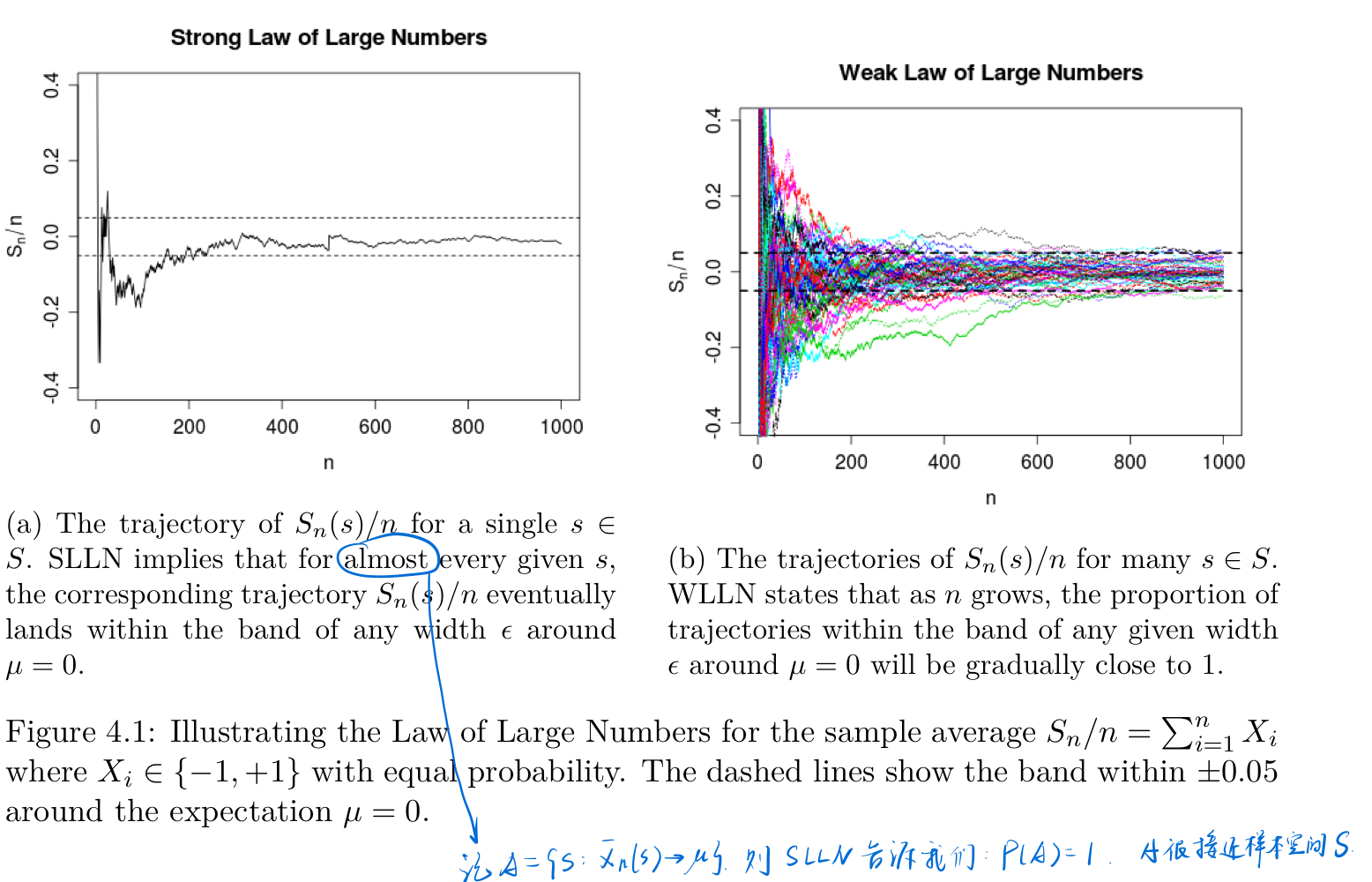
1. Strong law of large numbers: $P(\bar X_n\to \mu)=1$ (almost sure convergence $\bar X_n\overset{a.s.}{\to} \mu$ )
2. Weak law of large numbers: $\forall \epsilon > 0, P(|\bar X_n-\mu|>\epsilon)=0$ as $n\to \infty$ (convergence in probability $\bar X_n\overset{p}{\to} \mu$)

almost sure convergence implies convergence in probability.

Tail Probability Inequalities

Markov's
For any r.v. $X$ and constant $a>0$ ,

$$P(|X|>a)\le \frac{E|X|}{a}$$

Proof: Note that

$$|X|=|X|I(|X|>a)+|X|I(|X|<a)\ge aI(|X|>a)$$

take expectations on both side, then one can get the proof.

Chebyshev's

Let $X$ have mean $\mu$ and variance $\sigma^2$ . Then for any $a>0$,

$$P(|X-\mu|>a)\le \frac{\sigma ^2}{a^2}$$

CLT

Central Limit Theorem

Suppose that $X_1,...,X_n$ are $i.i.d.$ with finite mean $\mu$ and finite variance $\sigma ^2$ . Then

$$\lim_{n\to \infty}P \left( \frac{\bar X_n-\mu}{\sigma/\sqrt[]{n}}\le z \right)=\Phi(z),\quad \text{for any } z\in \mathbb{R}$$

(Convergence in distribution $\overset{d}{\to}$ )

Lyapunov's condition
Suppose that $X_1,...,X_n$ are independent with means $\mu_i$ and variances $\sigma_i^2$ . Let $s_n^2=\sum_{i=1}^n \sigma_i^2$ . Lyapunov's condition is that there exists $\delta >0$ such that

$$\lim_{n\to \infty} \frac{\sum_{i=1}^n E|X_i-\mu_i|^{2+\delta}}{s_n^{2+\delta}}=0.$$

分子是各随机变量的 $2+\delta$ 阶绝对中心矩的和，这刻画的是整个序列中存在至少一个随机变量出现极端值的潜能。而分母就是序列和的标准差的 $2+\delta$ 次方。比值趋于0，限制了序列中所有变量的波动程度。

Lyapunov's CLT

If Lyapunov's condition holds, then for $n\to \infty$

$$\frac{T-\mu_T}{s_n}\overset{d}{\to} N(0,1)$$

where $T=X_1+\cdots+X_n$ and $\mu_T=\sum_{i=1}^n \mu_i$.

参数估计

矩估计

矩是参数的函数 $\overset{\text{反解}}{\rightarrow}$ 参数是矩的函数 $\overset{\text{plug in 样本矩}}{\rightarrow}$ 得到估计量。

记 $\theta = g(\bm \mu)$ 其中 $\bm\mu$ 是各阶矩，那 $\hat\theta=g(\hat{\bm\mu})$ 就是矩估计量。若 $g$ 光滑，那么这个估计量是一致的。

反解挺麻烦的。

极大似然估计

设 $L(\theta; \mathbf{x})$ 为样本 $\mathbf{X} = (X_1, \ldots, X_n)$ 在观察到 $\mathbf{x} = (x_1, \ldots, x_n)$ 时关于参数 $\theta \in \Theta$ 的似然函数。使得似然函数达到最大值的 $\theta$ 值，即

$$\hat{\theta} = \hat{\theta}(\mathbf{x}) \quad \text{满足} \quad L(\hat{\theta}; \mathbf{x}) = \max_{\theta \in \Theta} L(\theta; \mathbf{x}),$$

称为参数 $\theta$ 的最大似然估计值。相应的统计量 $\hat{\theta}(\mathbf{X})$ 称为参数 $\theta$ 的最大似然估计量。两者通常都缩写为 MLE(Maximum Likelihood Estimate/Estimator)。

注：$\theta$ 可以是向量。

• MLE的存在要求似然函数能在定义域上取得最大值
• MLE不一定唯一，似然函数的最大值点都是合理的MLE
• 计算MLE通常并不容易，能手算的情况一般是求一阶条件解方程。

MLE的不变性 若 $\hat{\theta}$ 是 $\theta$ 的 MLE，那么对于任何函数 $g$，$g(\hat{\theta})$ 是 $g(\theta)$ 的 MLE。（$\theta$ 可以是向量）

一般条件下，

1. MLE $\hat\theta$ 是一致估计量
2. $\hat\theta$ 有渐进正态分布：

$$\sqrt{n}(\hat\theta-\theta)\overset{d}{\to} N(0,1/I(\theta))\quad n\to\infty$$

其中 $I(\theta)$ 是 Fisher 信息量，定义如下：

$$I(\theta) = -\mathbb{E}\left[\frac{\partial^2}{\partial \theta^2} \log f(X;\theta)\right]$$

$f$ 是单个观测的概率密度函数。

▶

Fisher信息量为啥这么定义

信息量是 $\theta$ 的信息量。作为一个分布的参数，怎么定义它的信息量呢？它变一下，整个分布就巨变，算不算信息量大？就从这个角度定义。

先想想怎么量化分布的巨变，那就是概率密度函数的巨变，我们这个定义与分布无关，所以用相对变化量，也就是 $\theta$ 出现微小变化量 $\partial\theta$ 时，对应的概率值的相对变化量 $\frac{\partial f(x;\theta)}{f(x;\theta)}$ （先视 $x$ 为常数）。注意

$$\frac{\partial f(x;\theta)}{f(x;\theta)} = \left(\frac{\partial}{\partial \theta} \log f(x;\theta)\right)\partial\theta$$

所以我们着重研究 $\frac{\partial}{\partial \theta} \log f(x;\theta)$ ，现在考虑 $x$ 的随机性，这变动有正有负，不能求均值吧，所以求它的二阶矩 $\mathbb{E}\left[\left(\frac{\partial}{\partial \theta} \log f(X;\theta)\right)^2\right]$，这个量越大，说明 $\theta$ 的微小变动引起的分布变动越大，所以信息量越大。这跟上面的定义一样，下面给出证明：

首先列出下面两个式子：

$$\begin{align*} \frac{\partial\log f}{\partial \theta}&=\frac{1}{f}\frac{\partial f}{\partial \theta}\\ \frac{\partial^2 \log f}{\partial \theta^2} &= \frac{\partial^2 f}{\partial \theta^2}\frac{1}{f}-(\frac{\partial f}{\partial \theta})^2 \frac{1}{f^2} \end{align*}$$

开始计算：

$$\begin{align*} \mathbb{E}\left[\left(\frac{\partial}{\partial \theta} \log f(X;\theta)\right)^2\right]&= \int \left(\frac{\partial}{\partial \theta} \log f(X;\theta)\right)^2 fdx \\ &= \int (\frac{\partial f}{\partial \theta})^2 \frac{1}{f} dx\\ &= \int \frac{\partial^2 f}{\partial \theta^2}-\frac{\partial^2 \log f}{\partial \theta^2}fdx\\ &= \int \frac{\partial^2 f}{\partial \theta^2} dx -\mathbb{E}\left[\frac{\partial^2}{\partial \theta^2} \log f(X;\theta)\right] \end{align*}$$

下面证明 $\int \frac{\partial^2 f}{\partial \theta^2} dx=0$，记得我的假设 $f$ 的性质足够好：

$$\begin{align*} \int \frac{\partial^2 f}{\partial \theta^2} dx&=\frac{\partial^2}{\partial \theta^2}\int fdx\\ &=\frac{\partial^2}{\partial \theta^2} 1 \\ &=0 \end{align*}$$

上面我们像物理学家一样随意玩弄了微分式，我们跟对待实数一样对待微元 $\partial f, \partial \log f, \partial \theta$ 。我们不应该厌弃这种做法，这对建立直觉很有帮助，当然了，不要泛滥，直觉有时也很不可靠。面临困难的问题时有正确的直觉，在直觉可能有错误时敏锐地发现，我想这是优秀的数学家具备的特质。

Cramer-Rao Lower Bound 设 $X_1,...,X_n$ 独立同分布，该分布依赖于一个未知参数 $\theta$，在一般条件下，任何 $\theta$ 的无偏估计量 $T(X_1,...,X_n)$ 的方差都满足

$$\operatorname{Var}(T)\ge \frac{1}{nI(\theta)}$$

一些例子

$X_1,...,X_n$ 独立同分布，服从均匀分布 $U(\theta, \theta + 1)$，请提出两个 $\theta$ 的无偏估计量，并讨论两者的有效性。

▶

解

求一阶矩为 $E(X_i)=\theta +\frac{1}{2}$，容易提出一个无偏估计量 $\hat{\theta}_1 = \bar X-\frac{1}{2}$. 其方差为 $\frac{1}{12n}$

容易发现样本均值是在估计取值取件的中点，即 $\theta +\frac{1}{2}$ ，对于中点的估计，我们有个老生常谈的讨论：均值还是中位数，仿照这个思路，我们提出

$$\hat\theta_2 = \frac{X_M+X_m-1}{2}$$

其中 $X_M=\max\{X_1,...,X_n\}, X_m=\min\{X_1,...,X_n\}$

先计算 $(X_M,X_m)$ 的联合密度函数 $g(u,v):$

$g(u,v)dudv$ 意即最大值与最小值分别落在 $u,v$ 附近，其他点落在 $(v,u)$ 区间内，这个值具体为

$$\binom{n}{n-2}\cdot 2\cdot f(u)duf(v)dv\cdot (F(u)-F(v))^{n-2}$$

前面的系数意为，从 $n$ 个点中选 $n-2$ 作为中间点，再从剩下的两个点中选最大值点。

代入 $f(x)=1, F(x)=x-\theta$ ，并消去 $dudv$ 得

$$g(u,v)=n(n-1)(u-v)^{n-2}$$

容易求得 $E(X_M)=\frac{n}{n+1}+\theta, E(X_m)=\frac{1}{n+1}+\theta$，无偏性容易验证。下面看这个估计量的方差：

算了以后再补，总之结果是 $\frac{1}{2(n+1)(n+2)}$，比上面那个好。

无偏性与一致性互不蕴含的几个例子

无偏但不一致

设 $X_1,X_2,\dots$ 独立同分布，满足 $E(X_i)=\mu$，$\operatorname{Var}(X_i)=\sigma^2<\infty$。

取估计量

$$T_n=X_1.$$

则

$$E(T_n)=E(X_1)=\mu,$$

所以它是无偏的，但显然它不一致。

一致但有偏

例1

用 $\frac{1}{n}\sum (X_i-\bar X)^2$ 估计总体方差

设 $X_1,\dots,X_n$ 独立同分布，均值为 $\mu$，方差为 $\sigma^2$。考虑估计量

$$T_n=\frac{1}{n}\sum_{i=1}^n (X_i-\bar X)^2.$$

它是我们熟悉的“样本方差的有偏版本”。其期望为

$$E(T_n)=\frac{n-1}{n}\sigma^2,$$

但它满足

$$T_n \xrightarrow{P} \sigma^2,$$

因此它是一致估计量。

例2

均匀分布 $U(0,\theta)$ 中用样本最大值估计上界

设 $X_1,\dots,X_n$ 独立同分布于 $U(0,\theta)$，其中 $\theta>0$ 未知。令

$$T_n=\max\{X_1,\dots,X_n\}.$$

则

$$P(T_n<t) = P(X_1<t)\cdots P(X_n<t)=\left(\frac{t}{\theta}\right)^n$$

因此

$$E(T_n)=\frac{n}{n+1}\theta,$$

有偏。

但是，对任意 $\varepsilon>0$，

$$P(|T_n-\theta|>\varepsilon)=P(T_n<\theta-\varepsilon) =\left(\frac{\theta-\varepsilon}{\theta}\right)^n \to 0,$$

所以

$$T_n \xrightarrow{P} \theta.$$

一致。

直觉修正

以上例子似乎在说，若估计量有偏但一致，那么期望的极限一定是真实参数值。这似乎有道理，对应的直觉是：在极限的世界里，估计量以1的概率取真实值，那它的期望肯定就是真实值咯。但是，这个直觉是错的。 考虑下面的例子：

真实参数 $\theta=0$，估计量取

$$\hat{\theta}_n = \begin{cases} n &\text{概率 } \frac{1}{n} \\ 0 &\text{概率 } 1-\frac{1}{n} \end{cases}$$

但 $\mathbb{E}(\hat{\theta}_n)=1$ ，而 $\hat{\theta}_n \xrightarrow{P} 0$。

上面的直觉错在哪里了呢？在于它先进入了极限的世界，再取期望，相当于做 $\mathbb{E}(\lim \hat\theta _n)$ （这不严谨，应该是依概率的极限，但无妨，我们会意即可） 的操作，但是我们的断言是 $\lim\mathbb{E}(\hat \theta _n)=\theta$ 。我们不加证明地让极限操作穿过了期望操作，这是有问题的，尽管对于性质良好的随机变量，这是合法的。

引用一位知乎上数学博主的话，数学概念的辨析，很多时候就是两个符号交换位置的意义辨析，很多错误的直觉就来自于鲁莽地交换符号的位置，上面的例子是 $\int_{}^{}$ 与 $\lim$ 符号，除此之外，还有 $\forall$ 和 $\exists$ 符号。

计量中的内生性

如何理解内生性

考虑下面的模型：

$$y = \beta_0 + \beta_1 x + u$$

我们说变量 $x$ 有内生性，是说 $Cov(x,u)\ne 0$，我们知道 $E(u\mid x)=0\Rightarrow Cov(x,u)=0$ ，所以此时 $u$ 的条件期望不再是常数，而是与 $x$ 相关的函数。对上面的模型两边同时取 $x$ 的条件期望，得

$$E(y\mid x) = \beta_0 + E(u\mid x) + \beta_1 x$$

假设 $E(u\mid x)$ 是关于 $x$ 的线性函数，那么

$$E(y\mid x) = \tilde\beta_0 + \tilde\beta_1 x$$

OLS 总是在估计 $x$ 对 $y$ 的最佳线性预测，也就是线性投影，也就是说它在估计 $\tilde\beta_0,\tilde\beta_1$ ，所以如果我们盲目地使用 OLS 来估计 $\beta_0,\beta_1$ ，那一定是有偏的。

---

我们对 $\beta_1$ 的理解，仍然可以是 “保持其他所有因素($u$)不变，$x$ 带来的边际影响”，而 OLS 估计的 $\tilde{\beta}_1$ 则混杂了由 $u$ 传导的影响，并不是 $x$ 的纯净影响。

内生性破坏了 OLS 对真实影响 $\beta_1$ 的识别能力。

如何检验内生性

假设我们怀疑 $X_1$ 是内生的，要做检验，必须要有一个合法的（或者我们相信是合法的）工具变量 $Z_1$ 。

第一个方法就是对比 $OLS$ 和 $2SLS$ 的系数。

第二个方法是用所有的外生变量和工具变量对 $X_1$ 做回归：

$$X_1 = \alpha_0 + \alpha_1 Z + \alpha_2 X_2 + v$$

$v$ 就是内生部分，用把估计的残差 $\hat v$ 作为新变量加入到模型中：

$$Y = \beta_0 + \beta_1 X_1 + \beta_2 X_2 + \gamma \hat{v} + e$$

检验 $\hat v$ 的系数，若显著不为零，则相信 $X_1$ 的内生的。

如何检验工具变量是合法的

弱工具变量检验

工具变量必须是外生的，且要和对应的内生变量相关。当工具变量刚好够用时，我们只能检验它与内生变量的相关性，因为根据OLS的代数性质，2SLS的残差 $\hat u$ 与工具变量 $z$ 必定满足 $\sum z_i\hat u_i=0$。

下面讲怎么检验相关性，这个检验对单一工具变量或者多工具变量都能用。做第一阶段回归：

$$x_1 = \pi_0 + \pi_1 z_1 + \pi_2 z_2 + \pi_3 x_2 +v$$

用 $F$ 检验

$$H_0: \pi_1 = \pi_2 =0$$

也就是检验工具变量的系数是否全为零。一般要求 $F>10$ 。

过度识别检验

英文是Over-identification Test，放个图：

假设检验

ANOVA

假设有 $I$ 组数据，每一组数据都从同方差的正态总体的简单随机样本。即

$$X_{ij}\sim N(\mu_i,\sigma^2)\quad \text{given } j, X_{ij}'s \text{ are i.i.d.}$$

下面给出一些定义：

总方差 $SST = \sum_i\sum_j (X_{ij}-\bar X_{..})^2$

组间方差 $SSTr = \sum_i\sum_j (\bar X_{i.}-\bar X_{..})^2$

组内方差之和 $SSE = \sum_i\sum_j (X_{ij}-\bar X_{i.})^2$

一个基础的关系：

$$SST = SSTr + SSE$$

两个重要结论:

1. $SSE/\sigma^2$ 服从自由度为 $IJ-1$ 的卡方分布
2. $\frac{SSTr/(I-1)}{SSE/(IJ-1)}$ 服从自由度为 $(I-1,IJ-1)$ 的 $F$ 分布

有了以上结论，就可以做 $F$ 检验：

$$\begin{align*} H_0&: \mu_1 = ... = \mu_I\\ H_a&: o.w \end{align*}$$

卡方检验

Pearson 卡方检验

观测 $N$ 个样本，共有 $k$ 类，每类频数为 $N_1,...,N_k$。

原假设：每一类样本出现的概率为 $p_1,...,p_k$ ；

备择假设：其他情况。

$H_0$ 下，期望频数 $E_i = Np_i$ ，观测频数 $O_i = N_i$ ，统计量

$$X^2 = \sum_{i=1}^k \frac{(O_i-E_i)^2}{E_i}$$

可以证明，$n\to \infty$ 时，$X^2\overset{d}{\to}\chi^2_{k-1}$。

应用：检验色子是否均匀。