线性回归分析-HW2

Prob-1

$$\hat{\beta}_1^{OLS}=\frac{\sum_{i=1}^{N}(x_i-\bar{x})(y_i-\bar{y})}{\sum_{i=1}^{N} (x_i-\bar{x})^{2}}$$

$$\hat{\beta}_0^{OLS}=\bar{y}-\hat{\beta}_1\bar{x}$$

Prob-2

$$\begin{align} \hat{\beta}_{0}^{ML},\hat{\beta}_{1}^{ML} &= \hat{\beta}_{0}^{LS},\hat{\beta}_{1}^{LS} \\ \hat{\sigma}^{2,ML}&=\frac{\sum e_{i}^{2}}{n} \end{align}$$

Prob-3

1.29

It means that the expected value of $Y$ is 0 given $X=0$. The curve of the function passes $(0,0)$ on a graph.

1.41

a.

Solve

$$\operatorname*{argmin}_{\hat{\beta}_1}\sum_{i=1}^{n} (y_i-\hat{\beta}_1x_i)^{2}$$

we get

$$\hat{\beta}_1^{OLS}=\frac{\sum_{i=1}^{n}x_iy_i}{\sum_{i=1}^{n} x_i^{2}}$$

b.

$$\begin{align} L(\beta_1\mid \boldsymbol{X},\boldsymbol{Y}) & =\prod_{i=1}^{n} f_{Y_i}(y_i\mid \beta_1,\sigma^{2},\boldsymbol{X}) \\ & = \cdots \exp \left( -\frac{1}{2\sigma^{2}}\sum_{i=1}^{n} (y_i-\beta_1x_i)^{2} \right) \end{align}$$

$\hat{\beta}^{ML}_1=\operatorname{argmax}_{\beta_1}L(\beta_1\mid \boldsymbol{X},\boldsymbol{Y})=\operatorname{argmin}_{\beta_1}\sum_{i=1}^{n} (y_i-\beta_1x_i)^{2}=\hat{\beta}_1^{OLS}$

It's the same as the least square estimator.

c.

$$\begin{align} \mathbb{E}\hat{\beta}_1^{ML} &= \mathbb{E}\left[ \frac{\sum_{i=1}^{n}x_iy_i}{\sum_{i=1}^{n} x_i^{2}} \right] \\ & = \frac{1}{\sum_{i=1}^{n} x_i^{2}}\mathbb{E}\left[ \sum_{i=1}^{n} x_i(\beta_1x_1+\varepsilon_i) \right] \\ & = \frac{1}{\sum_{i=1}^{n} x_i^{2}}\sum_{i=1}^{n} \left( \beta_1x_i^{2}+x_i\mathbb{E}\varepsilon_i \right) \\ & = \beta_1 \end{align}$$

Prob-4

a.

No. I don't know the exact distribution of $\varepsilon$.

b.

$Y=100+20\cdot 5+\varepsilon$ where $\varepsilon\sim N(0,25)$, so

$$P(195<Y<205)=P(-5<\varepsilon<5)=\Phi(1)-\Phi(-1)$$

where $\Phi(\cdot)$ is the CDF of standard normal distribution.

Prob-5

a.

The data obtained in the study were observational data because no experiment was made.

b.

It is not very valid. Relationship does not mean causality.

c.

Age, occupation

d.

Add more variables into the regression so that the error term has zero expectation. Or use instrumental variables to get the real effect.

Prob-6

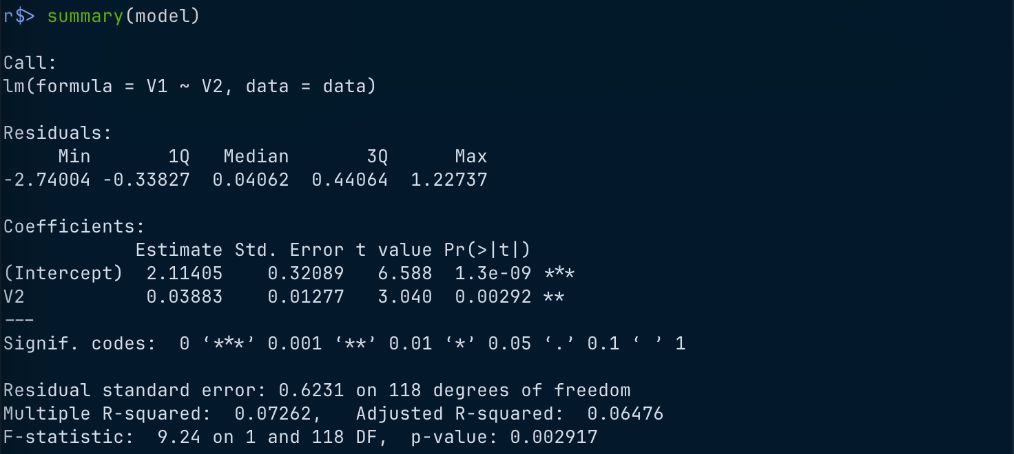
a.

$$\hat{\beta}_0=2.11,\, \hat{\beta}_1=0.039$$

The estimated regression function is

$$\hat{y}=2.11+0.039x$$

b.

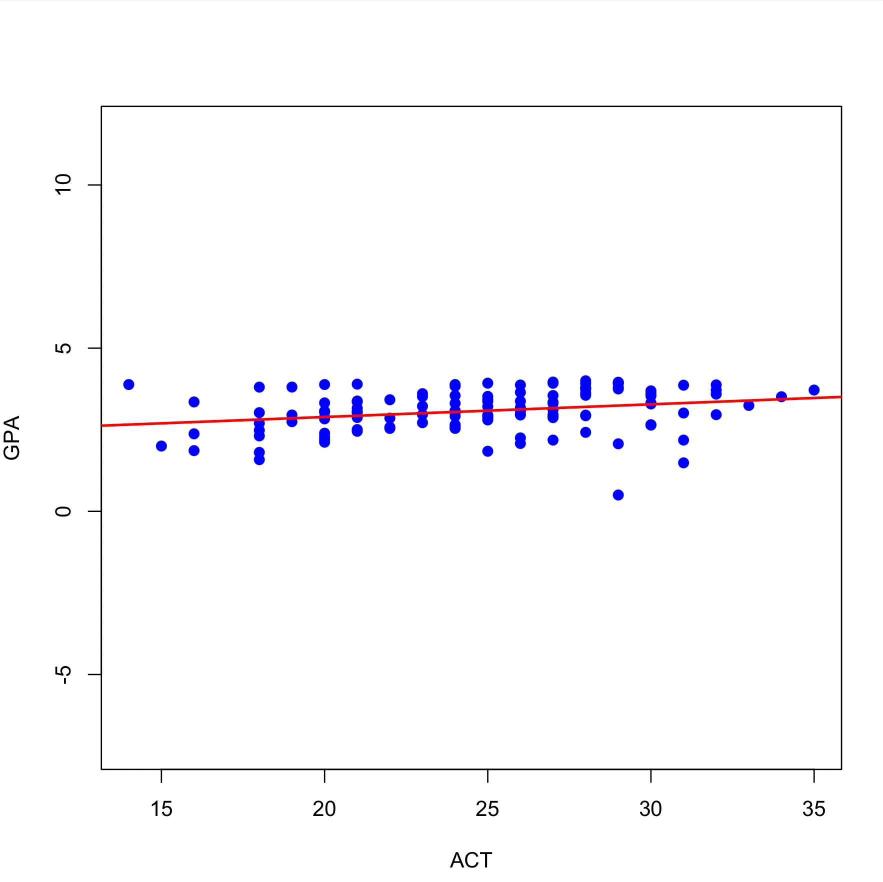
It seems good.

c.

3.278863

d.

0.038.