Prob-1
1-a
H 0 : β 1 = 3 H a : β 1 ≠ 3 \begin{align}
H_0 & : \beta_{1}=3 \\
H_a & : \beta_1\neq 3
\end{align}
H 0 H a : β 1 = 3 : β 1 = 3
the statistic is
t = β ^ 1 − 3 s ( β ^ 1 ) ∼ H 0 t 22 t=\frac{\hat{\beta}_1-3}{s(\hat{\beta}_{1})}\overset{H_0}{\sim}t_{22}
t = s ( β ^ 1 ) β ^ 1 − 3 ∼ H 0 t 22
we know from the table that
β ^ 1 = 3.5702 , s ( β ^ 1 ) = 0.347 \hat{\beta}_{1}=3.5702,\ s(\hat{\beta}_{1})=0.347
β ^ 1 = 3.5702 , s ( β ^ 1 ) = 0.347
so t = 1.643228 t=1.643228 t = 1.643228
The decision rule is
∣ t ∣ > ∣ t 0.975 , 23 ∣ = 2.068658 |t|>|t_{0.975,23}|=2.068658
∣ t ∣ > ∣ t 0.975 , 23 ∣ = 2.068658
So the conclusion is that we don't have enough evidence to say that the increase in the expected number of work hours in the Toluca Company does not equal this standard.
1-b
p o w e r ( 3.5 ) = P ( ∣ β ^ 1 − 3 s ( β ^ 1 ) ∣ > t 0.975 , 22 ∣ β 1 = 3.5 ) \mathrm{power}(3.5)=P(\left| \frac{\hat{\beta}_1-3}{s(\hat{\beta}_{1})} \right|>t_{0.975,22} \mid \beta_{1}=3.5)
power ( 3.5 ) = P ( s ( β ^ 1 ) β ^ 1 − 3 > t 0.975 , 22 ∣ β 1 = 3.5 )
Because when β 1 = 3.5 \beta_{1}=3.5 β 1 = 3.5
β ^ 1 − 3 s ( β ^ 1 ) ∼ t ( 23 , 0.5 σ ( β ^ 1 ) ) \frac{\hat{\beta}_1-3}{s(\hat{\beta}_{1})} \sim t\left( 23, \frac{0.5}{\sigma(\hat{\beta}_{1})} \right)
s ( β ^ 1 ) β ^ 1 − 3 ∼ t ( 23 , σ ( β ^ 1 ) 0.5 )
so
p o w e r ( 3.5 ) = 0.277781 \mathrm{power}(3.5)=0.277781
power ( 3.5 ) = 0.277781
1-c
F ∗ F^{*} F ∗
H 0 ′ : β 1 = 0 H_0':\beta_{1}=0
H 0 ′ : β 1 = 0
the null hypothesis is different.
Prob-2
2-a
2-b
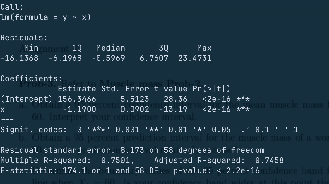
1.19
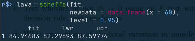
84.94683
4.4432518
8.173
Prob-3
3-a
s 2 = M S E ⋅ [ 1 n + ( X h − X ˉ ) 2 S x x ] = 8.173 ⋅ [ 1 60 + ( 60 − 59.98333 ) 2 8210.983 ] = 0.1362194 s^{2}=MSE\cdot\left[ \frac{1}{n}+ \frac{(X_{h}-\bar{X})^{2}}{S_{x x}} \right]=8.173\cdot\left[ \frac{1}{60}+\frac{(60-59.98333)^{2}}{8210.983} \right]=0.1362194
s 2 = M S E ⋅ [ n 1 + S xx ( X h − X ˉ ) 2 ] = 8.173 ⋅ [ 60 1 + 8210.983 ( 60 − 59.98333 ) 2 ] = 0.1362194
CI:
84.94683 ± s ⋅ t 0.975 , 58 = [ 84.81061 , 85.08305 ] 84.94683\pm s\cdot t_{0.975,58} = [84.81061,85.08305]
84.94683 ± s ⋅ t 0.975 , 58 = [ 84.81061 , 85.08305 ]
3-b
s 2 = M S E ⋅ [ 1 + 1 n + ( X h − X ˉ ) 2 S x x ] = 8.173 ⋅ [ 1 + 1 60 + ( 60 − 59.98333 ) 2 8210.983 ] = 8.309219 s^{2}=MSE\cdot\left[ {\color{red}1+}\frac{1}{n}+ \frac{(X_{h}-\bar{X})^{2}}{S_{x x}} \right]=8.173\cdot\left[ 1+\frac{1}{60}+\frac{(60-59.98333)^{2}}{8210.983} \right]=8.309219
s 2 = M S E ⋅ [ 1 + n 1 + S xx ( X h − X ˉ ) 2 ] = 8.173 ⋅ [ 1 + 60 1 + 8210.983 ( 60 − 59.98333 ) 2 ] = 8.309219
CI:
84.94683 ± s ⋅ t 0.975 , 58 = [ 76.63761 , 93.25605 ] 84.94683\pm s\cdot t_{0.975,58} = [76.63761,93.25605]
84.94683 ± s ⋅ t 0.975 , 58 = [ 76.63761 , 93.25605 ]
3-c
Yes it is wider and it should be wider.
Prob-4
4-a
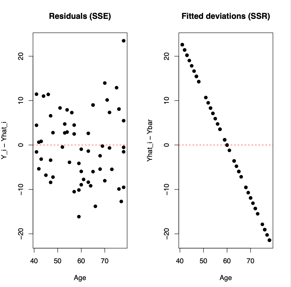
SSR seems to be larger. This implies that R 2 > 0.5 R^{2}>0.5 R 2 > 0.5
4-b
4-c
H 0 : β 1 = 0 H a : β 1 ≠ 0 \begin{align}
H_0 & : \beta_{1}=0 \\
H_a & : \beta_{1}\ne 0
\end{align}
H 0 H a : β 1 = 0 : β 1 = 0
Decision rule:
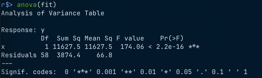
F > F 0.95 , 1 , 58 F>F_{0.95,1,58}
F > F 0.95 , 1 , 58
Conclusion: Reject.
4-d
R 2 = 0.7501 R^{2}=0.7501 R 2 = 0.7501 ≈ 25 % \approx 25\% ≈ 25%
4-e
R 2 = 0.750 , r = − 0.866 R^{2}= 0.750,\quad r = −0.866 R 2 = 0.750 , r = − 0.866
Prob-5
5-a
E [ M S R ] = σ 2 + β 1 2 S x x = 1026.36 E [ M S E ] = σ 2 = 0.36 \begin{align}
\mathbb{E}[MSR] & =\sigma^{2}+\beta_{1}^{2}S_{x x} = 1026.36\\
\mathbb{E}[MSE] & =\sigma^{2}=0.36
\end{align}
E [ M S R ] E [ M S E ] = σ 2 + β 1 2 S xx = 1026.36 = σ 2 = 0.36
5-b
S x x S_{x x} S xx
The mean response for X = 8 X=8 X = 8
0.36 ⋅ [ 1 5 + ( 8 − 8 ) 2 114 ] , 0.36 ⋅ [ 1 5 + ( 8 − 8 ) 2 10 ] 0.36\cdot\left[ \frac{1}{5}+ \frac{(8-8)^{2}}{114} \right],\ 0.36\cdot \left[ \frac{1}{5}+ \frac{(8-8)^{2}}{10} \right]
0.36 ⋅ [ 5 1 + 114 ( 8 − 8 ) 2 ] , 0.36 ⋅ [ 5 1 + 10 ( 8 − 8 ) 2 ]
they are the same. So both sets of observations are OK. But if it is not for X = 8 X=8 X = 8
Prob-6
E ( Y i − Y ˉ ) 2 = E ( β 1 ( X i − X ˉ ) + ε i − ε ˉ ) 2 = β 1 2 ( X i − X ˉ ) 2 + n − 1 n σ 2 \begin{align}
\mathbb{E}(Y_{i}-\bar{Y})^{2} & = \mathbb{E}(\beta_{1}(X_{i}-\bar{X})+\varepsilon_{i}-\bar{\varepsilon})^{2} \\
& = \beta_{1}^{2}(X_i-\bar{X})^{2}+ \frac{n-1}{n}\sigma^{2}
\end{align}
E ( Y i − Y ˉ ) 2 = E ( β 1 ( X i − X ˉ ) + ε i − ε ˉ ) 2 = β 1 2 ( X i − X ˉ ) 2 + n n − 1 σ 2
so
E ( ∑ ( Y ^ i − Y ˉ ) 2 ) = β 1 2 S x x + ( n − 1 ) σ 2 \mathbb{E}\left( \sum (\hat{Y}_{i}-\bar{Y})^{2} \right)=\beta_{1}^{2}S_{x x}+(n-1)\sigma^{2}
E ( ∑ ( Y ^ i − Y ˉ ) 2 ) = β 1 2 S xx + ( n − 1 ) σ 2
instead of ( n − 1 ) σ 2 (n-1)\sigma^{2} ( n − 1 ) σ 2