3 Statistical Inference and Power

Recap on Inference

Sampling Distribution

抽样分布:一个统计量,比如样本均值、样本方差,是根据样本计算得出的,而得到的样本是有随机性的。假设我们回到过去,重新抽样一次,可以想象,抽样的结果会是不同的。因此根据样本计算的统计量也是有随机性的,这些统计量的分布就是抽样分布。

Sampling Distribution of Mean of Normal Population

样本量为 nn,简单随机抽样(即样本间独立同分布)出 X1,…,XnX_{1},\dots,X_{n},总体分布为 N(μ,σ2)N(\mu,\sigma^{2}),则

Xˉ∼N(μ,σ2n)\bar{X}\sim N\left( \mu, \frac{\sigma^{2}}{n} \right)

记 s2=∑(Xi−Xˉ)2n−1s^{2}=\frac{\sum(X_{i}-\bar{X})^{2}}{n-1},则 σ^2(Xˉ)=s2n\hat{\sigma}^{2}(\bar{X})=\frac{s^{2}}{n},sn\frac{s}{\sqrt{n}} 称为 Xˉ\bar{X} 的标准误。

注意这里的标准误是一个估计量,即可以从手头的数据计算得到。

事实上,wiki 百科给出的标准误的定义为

The standard error (SE) of a statistic is the standard deviation of its sampling
distribution

而不是估计版本,但是实践上似乎不怎么区分两者。

Sampling Distribution of Variance of Normal Population

见 概统拾遗 › ^sampling-dist-of-sample-variance,可以证明

(n−1)s2σ2=Z12+⋯+Zn−12\frac{(n-1)s^{2}}{\sigma^{2}}=Z_{1}^{2}+\cdots+Z_{n-1}^{2}

其中 Z1,…,Zn−1∼i.i.d.N(0,1)Z_{1},\dots,Z_{n-1}\overset{i.i.d.}{\sim}N(0,1)

因此

(n−1)s2σ2∼χn−12\frac{(n-1)s^{2}}{\sigma^{2}}\sim \chi^{2}_{n-1}

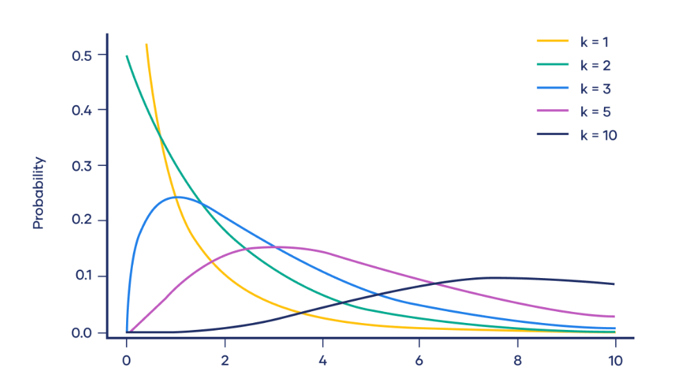
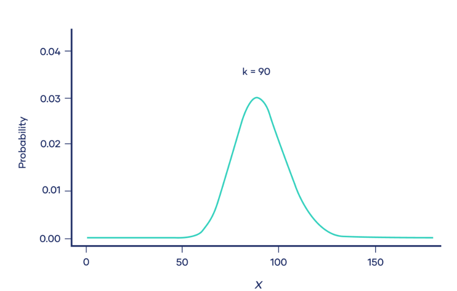
The Chi-Square Distribution

可以发现,自由度大于 2 后,会呈现峰型。当自由度大于 90 后,就非常像正态分布了。

Fisher's Theorem

正态总体下,简单随机抽样的样本均值与样本方差独立。

证明见 概统拾遗 › ^sample-mean-and-sample-variance

Student's t-distribution

Consider

U∼χk2Z∼N(0,1)U⊥Z\begin{align} U & \sim \chi^{2}_k \\ Z & \sim N(0,1) \\ U & \perp Z \end{align}

then

ZU/k∼tk\frac{Z}{\sqrt{U/k}}\sim t_k

Applying this result, we have

T=Xˉ−μs/n∼tn−1T=\frac{\bar{X}-\mu}{s/\sqrt{n}}\sim t_{n-1}

Inference in SLR

Inference Concerning β1\beta_1

LS estimator b1=SxySxxb_1=\frac{S_{xy}}{S_{xx}}. Expanding SxyS_{xy} yields

b1=β1+∑Xi−XˉSxxεib_1 = \beta_1 + \sum \frac{X_i-\bar{X}}{S_{xx}}\varepsilon_i

so

E[b1]=β1V[b1]=σ2Sxx\begin{align} \mathbb{E}[b_1] & =\beta_1 \\ \mathbb{V}[b_1] & = \frac{\sigma^{2}}{S_{xx}} \end{align}

The expression of V[b1]\mathbb{V}[b_{1}] deserves closer examination. It says that larger error term variance makes it harder to estimate β1\beta_1, whereas a greater spread in the observed XiX_i's increases the precision of the estimator.

The unbiasedness of b1b_{1} uses the following assumption:

  • Zero conditional mean

The induction of V[b1]\mathbb{V}[b_1] uses the following assumptions:

  1. εi\varepsilon_i's are non-correlated
  2. Equal variances

It is easy to see that b1b_1 is normally distributed. So

b1−β1σ/Sxx∼N(0,1)\frac{b_1-\beta_1}{\sigma/\sqrt{S_{xx}}}\sim N(0,1)

And because s2=SSEn−2s^{2}=\frac{SSE}{n-2} satisfies

(n−2)s2σ2∼χn−22,s2⊥b1\frac{(n-2)s^{2}}{\sigma^{2}}\sim \chi^{2}_{n-2},\quad s^{2}\perp b_1

so

b1−β1s/Sxx∼tn−2\frac{b_1-\beta_1}{s/\sqrt{S_{xx}}}\sim t_{n-2}

We can use it to perform hypothesis testing and construct confidence intervals.

Chi-square distribution:

Let

X=(1X11X2⋮⋮1Xn)X=\begin{pmatrix} 1 & X_1 \\ 1 & X_2 \\ \vdots & \vdots \\ 1 & X_n \end{pmatrix}

Then Y^=HY\hat{Y}=HY, where

H=X(XTX)−1XTH=X(X^TX)^{-1}X^T

thus

e=Y−Y^=(I−H)Y=(I−H)(Xβ+ε)=(I−H)εe=Y-\hat{Y}=(I-H)Y=(I-H)(X\beta+\varepsilon)=(I-H)\varepsilon

where the last equality follows because I−HI-H is the orthogonal projection matrix onto R(X)⊥\mathcal{R}(X)^{\perp}.

So

SSE=eTe=εT(I−H)T(I−H)ε=εT(I−H)ε\color{blue} SSE=e^Te = \varepsilon^T(I-H)^T(I-H)\varepsilon= \varepsilon^T(I-H)\varepsilon

Since I−HI-H is symmetric and has rank n−2n-2, so there exists an orthogonal matrix QQ such that

I−H=QΛQTI-H = Q \Lambda Q^T

and because I−H=(I−H)2I-H=(I-H)^{2}, Λ=(In−2O)\Lambda = \begin{pmatrix}I_{n-2} & \\ & O\end{pmatrix}.

Note that εσ∼N(0,In)\frac{\varepsilon}{\sigma}\sim N(0,I_n) and orthogonal transformations preserve the joint standard normal distribution and hence the independence of its components (Cov(AX,BY)=ACov(X,Y)BT\mathrm{Cov}(AX,BY)=A\mathrm{Cov}(X,Y)B^T), so QTεσ∼N(0,In)Q^T \frac{\varepsilon}{\sigma}\sim N(0,I_n).

Finally,

(n−2)s2σ2=SSEσ2=Z12+⋯+Zn−22∼χn−22\frac{(n-2)s^{2}}{\sigma^{2}} = \frac{SSE}{\sigma^{2}} = Z_1^{2}+\dots+Z_{n-2}^{2}\sim \chi^{2}_{n-2}

where Zi∼i.i.d.N(0,1)Z_i \overset{i.i.d.}{\sim}N(0,1).

As for the independence, we can first see that b−β=(XTX)−1XTε,b-\beta = (X^TX)^{-1}X^T\varepsilon, which is a linear combination of εi\varepsilon_i's, and s2s^{2} is a function of (I−H)ε(I-H)\varepsilon which is also a linear combination of εi\varepsilon_i's. As εi∼i.i.d.N(0,1)\varepsilon_i \overset{i.i.d.}{\sim}N(0,1), b−β,(I−H)εb-\beta, (I-H)\varepsilon are jointly multivariate normal. So we only need to justify Cov(b−β,(I−H)ε)=0.\mathrm{Cov}(b-\beta,(I-H)\varepsilon)=0. Fortunately,

Cov(b−β,(I−H)ε)=(XTX)−1XT⋅σ2⋅(I−H)T=0\begin{align} \mathrm{Cov}(b-\beta,(I-H)\varepsilon) & = (X^TX)^{-1}X^T\cdot \sigma^{2} \cdot (I-H)^T \\ & = 0 \end{align}

because (I−H)X=O(I-H)X=O (projecting itself to its own orthogonal complement)

Testing Correlation

Let (xi,yi)(x_i,y_i) be a bivariate normal random sample of size nn, then

E[Y∣X=x]=(μY−ρσYσXμX)+ρσYσXx\mathbb{E}[Y\mid X=x] = \left( \mu_Y-\rho \frac{\sigma_Y}{\sigma_X} \mu_X\right)+ \rho \frac{\sigma_Y}{\sigma_X}x

Note that b1=SxySxx=SxySxxSyy⋅SyySxx=rσ^Yσ^Xb_1=\frac{S_{xy}}{S_{xx}}=\frac{S_{xy}}{\sqrt{S_{xx}S_{yy}}}\cdot \frac{\sqrt{S_{yy}}}{\sqrt{S_{xx}}}=r \frac{\hat{\sigma}_Y}{\hat{\sigma}_X},

Testing H0:ρ=0H_0: \rho=0 is equivalent to testing H0:β1=0H_0:\beta_1=0

We'll show in next lecture that

t=r1−r2n−2∼tn−2t=\frac{r}{\sqrt{1-r^{2}}}\sqrt{n-2}\sim t_{n-2}

More appropriate when it is not sure which variable is the response.

Inference Concerning β0\beta_0

Similarly, can show that

b0∼N(β0,σ2(b0))b_0\sim N(\beta_0,\sigma^{2}(b_0))

where

σ2(b0)=σ2⋅(1n+Xˉ2Sxx)\sigma^{2}(b_0)=\sigma^{2}\cdot\left( \frac{1}{n}+\frac{\bar{X}^{2}}{S_{xx}} \right)

t-statistic under H0:β0=0H_0:\beta_0=0

b0−0s(b0)∼tn−2\frac{b_0-0}{s(b_0)}\sim t_{n-2}

where

s(b0)=s1n+Xˉ2Sxxs(b_0)=s\sqrt{\frac{1}{n}+\frac{\bar{X}^{2}}{S_{xx}}}

Remarks

Inference concerning β0\beta_0 is usually not of interest, because shift in XX causes shift in β0\beta_0, and X=0X=0 may not be in the scope (the range of the explanatory variable).

Meme on the scope of the explanatory variable

OLS Estimators Are BLUE

For an independent random sample (Y1,…,Yn)(Y_1,\dots,Y_n) from a population with mean μ\mu, the sample mean Yˉ\bar{Y} was shown to be a best linear unbiased estimator of μ\mu.

b1b_{1} is BLUE

Let b1=∑ciYib_{1}=\sum c_{i}Y_{i}, where ci=Xi−XˉSxx.c_{i}=\frac{X_{i}-\bar{X}}{S_{xx}}.

Take any other linear estimator of β1\beta_{1}:

β~1=∑wiYi,wi=ci+di,\tilde\beta_1 = \sum w_i Y_i, \qquad w_i = c_i + d_i,

where did_{i} are arbitrary constants (functions of the XiX_{i}'s only).

Unbiasedness constraints.

E[β~1]=β0∑wi+β1∑wiXi.E[\tilde\beta_1] = \beta_0\sum w_i + \beta_1\sum w_iX_i.

For this to equal β1\beta_{1} for all β1,β0\beta_{1},\beta_{0} we need ∑wi=0\sum w_{i}=0 and ∑wiXi=1\sum w_{i}X_{i}=1. Since cic_{i} already satisfies these, we need

∑di=0,∑diXi=0.\sum d_i = 0, \qquad \sum d_i X_i = 0.

this lead to ∑cidi=0.\sum c_{i}d_{i}=0.

Variance.

Var(β~1)=σ2∑wi2=σ2[∑ci2+2∑cidi+∑di2]=σ2[1Sxx+∑di2].\text{Var}(\tilde\beta_1) = \sigma^2\sum w_i^2 = \sigma^2\left[\sum c_i^2 + 2\sum c_i d_i + \sum d_i^2\right] = \sigma^2\left[\frac{1}{S_{xx}} + \sum d_i^2\right].

Therefore

Var(β~1)=Var(β^1)+σ2∑di2  ≥  Var(b1),\text{Var}(\tilde\beta_1) = \text{Var}(\hat\beta_1) + \sigma^2\sum d_i^2 \;\ge\; \text{Var}(b_{1}),

with equality iff all di=0d_{i}=0, i.e., β~1=b1\tilde{\beta}_1=b_{1}.

b0b_{0} is BLUE

Let b0=∑aiYib_{0}=\sum a_{i}Y_{i}, where ai=1N+Xˉ(Xi−Xˉ)Sxxa_{i}=\frac{1}{N}+\frac{\bar{X}(X_{i}-\bar{X})}{S_{xx}}

Take any other linear estimator of β0\beta_{0}:

β~0=∑wiYi,wi=ai+di,\tilde\beta_0 = \sum w_i Y_i, \qquad w_i = a_i + d_i,

Similarly, unbiasedness requires

∑di=0,∑diXi=0.\sum d_i = 0, \qquad \sum d_i X_i = 0.

which leads to ∑aidi=0\sum a_{i}d_{i}=0

Let's see the variance:

V[β~0]=σ2∑(ai+di)2=σ2(∑ai2+∑di2)≥σ2∑ai2=V[b0]\mathbb{V}[\tilde{\beta}_{0}]=\sigma^{2}\sum (a_{i}+d_{i})^{2}=\sigma^{2}\left( \sum a_{i}^{2}+\sum d_{i}^{2} \right) \geq \sigma^{2}\sum a_{i}^{2}=\mathbb{V}[b_0]

The equality holds iff di=0 ∀id_{i}=0\ \forall i.

So b0b_{0} is the best among them.

Joint Inference of β0\beta_0 and β1\beta_1

Confidence region is used for two or more parameters.

P((β0,β1)∈S⊂R2)=100(1−α)%P\left( (\beta_0,\beta_1)\in S \subset \mathbb{R}^{2} \right) = 100(1-\alpha)\%

Since

(b0,b1)T∼N((β0,β1)T,σ2Σ)(b_0,b_1)^T\sim N\left( (\beta_0,\beta_1)^T,\sigma^{2}\Sigma \right)

the natural (i.e. smallest) confidence region is an ellipse. However, the textbook considers rectangles.

Simply combining individual CIs is not desired:

P(β0∈CI0)=1−α,P(β1∈CI1)=1−αP(\beta_0\in CI_0)=1-\alpha, \quad P(\beta_1 \in CI_1)=1-\alpha

Let

S=CI0×CI1S=CI_0\times CI_1

then

P((β0,β1)∈S)=P((β0∈CI0)∩(β1∈CI1))=1−P((β0∉CI0)∪(β1∉CI1))≤1−P(β0∉CI0)=1−α\begin{align} P((\beta_0,\beta_1)\in S) & = P((\beta_0\in CI_0) \cap (\beta_1\in CI_1)) \\ & = 1- P((\beta_0\notin CI_0) \cup (\beta_1\notin CI_1)) \\ & \leq 1-P(\beta_0 \not\in CI_0) \\ & =1-\alpha \end{align}


In order to achieve confidence level at least 1−α1-\alpha, set α0=α/2\alpha_0=\alpha/2, so

P(β0∈CI0)=1−α0,P(β1∈CI1)=1−α0P(\beta_0\in CI_0)=1-\alpha_0, \quad P(\beta_1 \in CI_1)=1-\alpha_0

and

P((β0,β1)∈S)=P((β0∈CI0)∩(β1∈CI1))=1−P((β0∉CI0)∪(β1∉CI1))≥1−[P(β0∉CI0)+P(β1∉CI1)]=1−α\begin{align} P((\beta_0,\beta_1)\in S) & = P((\beta_0\in CI_0) \cap (\beta_1\in CI_1)) \\ & = 1- P((\beta_0\notin CI_0) \cup (\beta_1\notin CI_1)) \\ & \geq 1-[P(\beta_0 \not\in CI_0)+P(\beta_1 \not\in CI_1)] \\ & =1-\alpha \end{align}

Power

The power of a significance test is the probability that the null hypothesis is correctly rejected.

  • power=1−P(Type II error)\mathrm{power}=1-P(\text{Type II error})
  • Depends on the particular value of the parameter in H1H_1
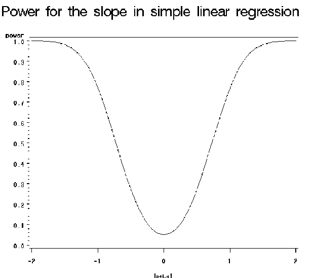
  • Often depicted by a curve as the value of the parameter in H1H_1 changes

Power for Testing β1\beta_1

Consider the test

H0:β1=0H1:β1≠0H_0:\beta_{1}=0\quad H_1:\beta_1\ne 0

power=power(β1)=P(reject H0∣H1 holds)=P(∣b1∣s(b1)>tn−2,1−α/2∣β1≠0)\mathrm{power}=\mathrm{power}(\beta_1)=P(\text{reject }H_0\mid H_1 \text{ holds}) = P\left( \frac{|b_1|}{s(b_1)}>t_{n-2,1-\alpha/2}\mid \beta_1 \ne 0 \right)

when β1=0\beta_1=0, we can just define the power as α\alpha so it is easy to compute the power. But when β1≠0\beta_1\ne 0, we don't know the distribution of

T=b1s(b1)T=\frac{b_{1}}{s(b_{1})}

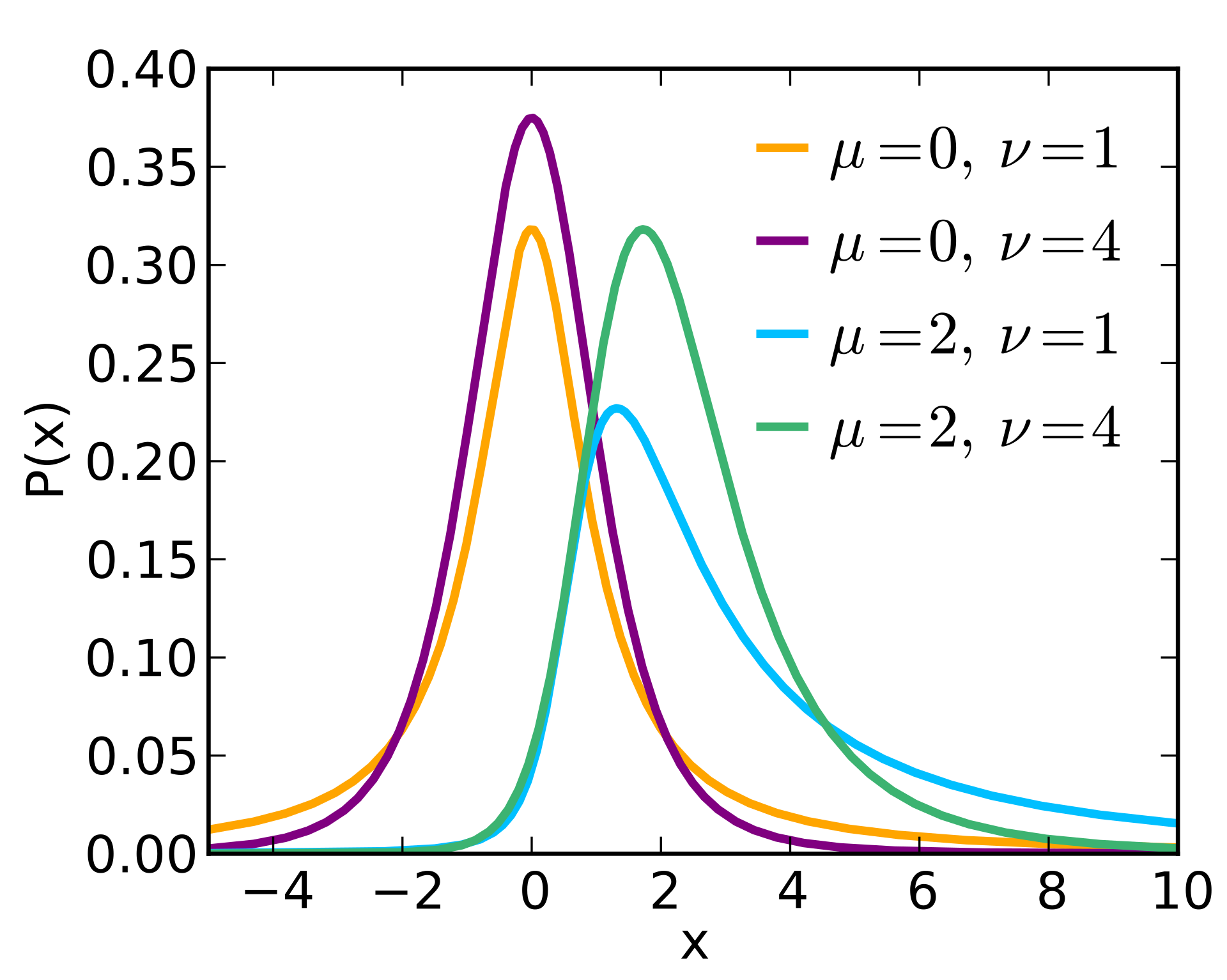
Non-Central tt-Distribution

First introduce the non-central tt-distribution:

If Z∼N(0,1),U∼χk2Z\sim N(0,1),U\sim \chi^{2}_{k}, and Z⊥UZ\perp U then

Z+δU/k∼t(k,δ)\frac{Z+\delta}{\sqrt{U/k}}\sim t(k,\delta)

which is a non-central tt-distribution with df kk and the non-centrality parameter δ\delta.

So

T=b1−β1+β1s(b1)∼t(n−2,β1σ(b1))T=\frac{b_{1}-\beta_{1}+\beta_{1}}{s(b_{1})}\sim t\left( n-2, \frac{\beta_{1}}{\sigma(b_{1})} \right)

With this we can compute power(β1)\mathrm{power}(\beta_{1}).

PDF of Non-Central t-Distribution

Note that the non-central t-distribution is asymmetric, however the asymmetry becomes smaller the larger degree of freedom.

In order to calculate power(β1)\mathrm{power}(\beta_{1}), we need to know or assume σ(b1)\sigma(b_{1}) from prior knowledge or pilot study.

Since

T=b1−β1s(b1)+β1s(b1)T=\frac{b_{1}-\beta_{1}}{s(b_{1})}+\frac{\beta_{1}}{s(b_{1})}

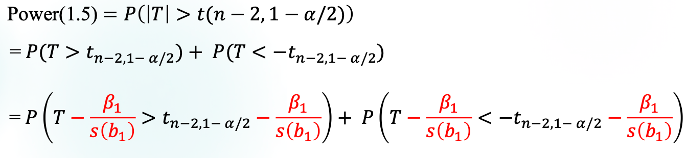
and the former part follows tn−2t_{n-2}, why don't we just calculate the power like following

?

The reason is that the term β1s(b1)\frac{\beta_{1}}{s(b_{1})} is an r.v.. Though the left part of the inequality follows tt-distribution, the randomness of the right part cannot be ignored.

How to Increase the Power

It is equivalent to ask when ∣b1∣s(b1)\frac{|b_{1}|}{s(b_{1})} is more likely to be large enough.

  • ∣b1∣|b_1| tends to be large when the non-centrality is significant, i.e., β1\beta_1 is far from the null value
  • s(b1)=sSxxs(b_{1})=\frac{s}{\sqrt{S_{xx}}} is small when SxxS_{xx} is large →\to increase the sample size.

Cov(Yˉ,b1)\mathrm{Cov}(\bar{Y},b_1) 一个上下,一个左右,随机性正交。


3 Statistical Inference and Power
https://wtx17.github.io/2026/09/29/Lec3-Statistical-Inference-and-Power/
作者
wtx
发布于
2026年9月29日
更新于
2026年11月6日
许可协议