5 Model Assumptions and Diagnostics

Lec5 slides.

线性回归模型的概率方面的假设都会体现在 $Y$ 的概率分布上，我们能否查看手头 $Y$ 样本的频率直方图来做诊断？

不能！见 LINE 假设，$Y_{i}$ 并不是独立同分布的。放一块看频率直方图不行。

xxx">Diagnostics Concerning $X$

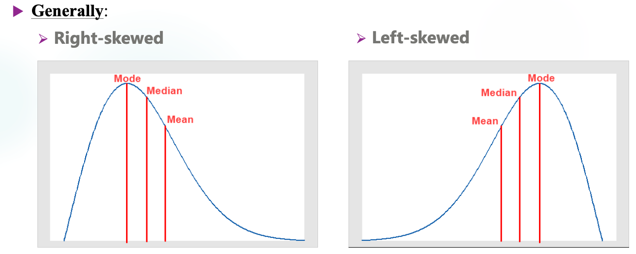
Skewness

$$g_{1}=\frac{m_{3}}{m_{2}^{3/2}}= \frac{\frac{1}{n}\sum(x_{i}-\bar{x})^{3}}{\left( \frac{1}{n}\sum (x_{i}-\bar{x})^{2} \right)^{3/2}}$$

• $g_{1}<0$: some data points lying in the left side of $\bar{x}$ are significant $\to$ skewed left/negative, the left tail is thicker.
• $g_{1}>0$: similar

Kurtosis

$$g_{2}=\frac{m_{4}}{m_{2}^{2}}-3= \frac{\frac{1}{n}\sum(x_{i}-\bar{x})^{4}}{\left( \frac{1}{n}\sum (x_{i}-\bar{x})^{2} \right)^{2}}-3$$

• $g_{2}=0$ for a normal distribution

• Sometimes referred to as the excess kurtosis, where as the one without $-3$ is called kurtosis.

  • In practice, note which one is used.

• $\dfrac{m_{4}}{m_{2}^{2}}\geq 1$.

• $g_{2}>0$: there are decent number of points lying very far from $\bar{x}\to$ heavy tail or we call leptokurtic distribution, where "lepto-" means "slender".

• $g_{2}<0$: platykurtic distribution where "platy-" means "broad". Light tails.

• Note that we are comparing with the normal distribution.

名字起得不好，实际看的不是峰而是尾。尖峰——厚尾，平峰——薄尾。

Kurtosis is scale free. It reflects the shape of a distribution apart from the variance.

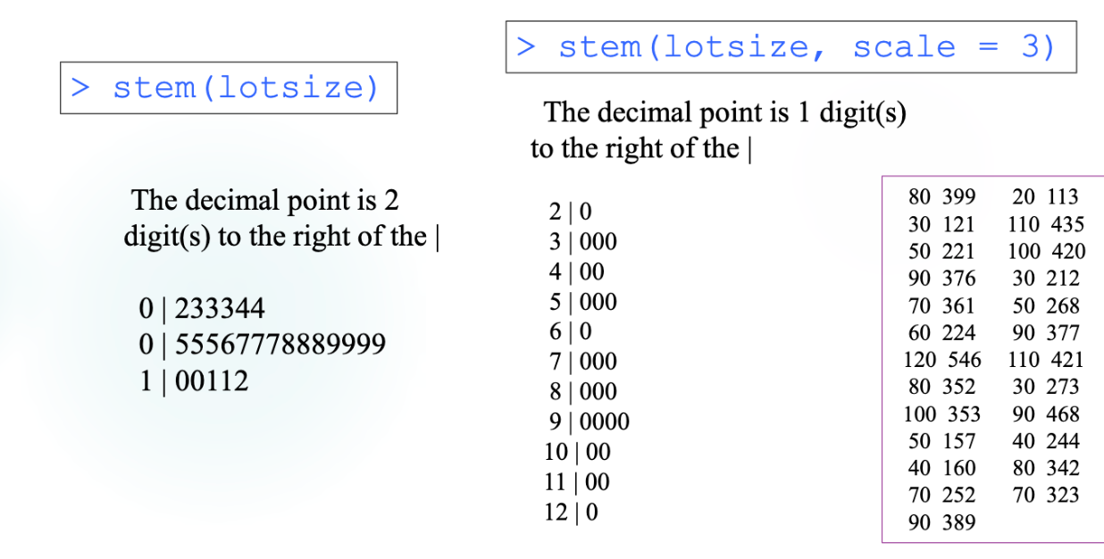
Stem-and-Leaf Plots

Useful to find the mode (众数).

Box Plots

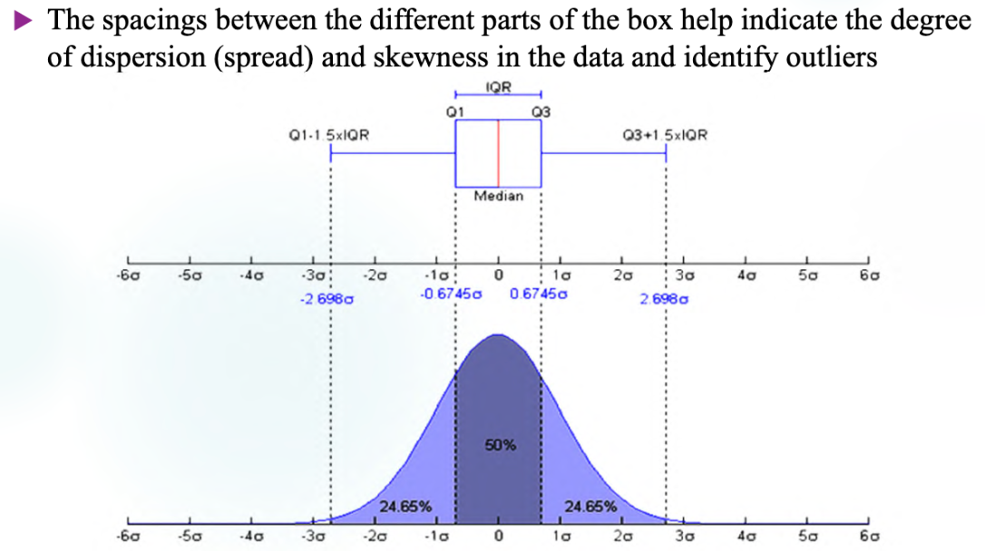
Important concepts:

• IQR $=Q_{3}-Q_{1}$.
• whiskers: $Q_{1}-1.5IQR$ and $Q_{3}+1.5IQR$.

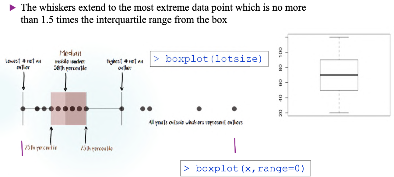
Note that whiskers always end at actual data points rather than at the calculated limits. The whisker instead ends at the most extreme observed data point within the calculated limit.

Histogram Plots

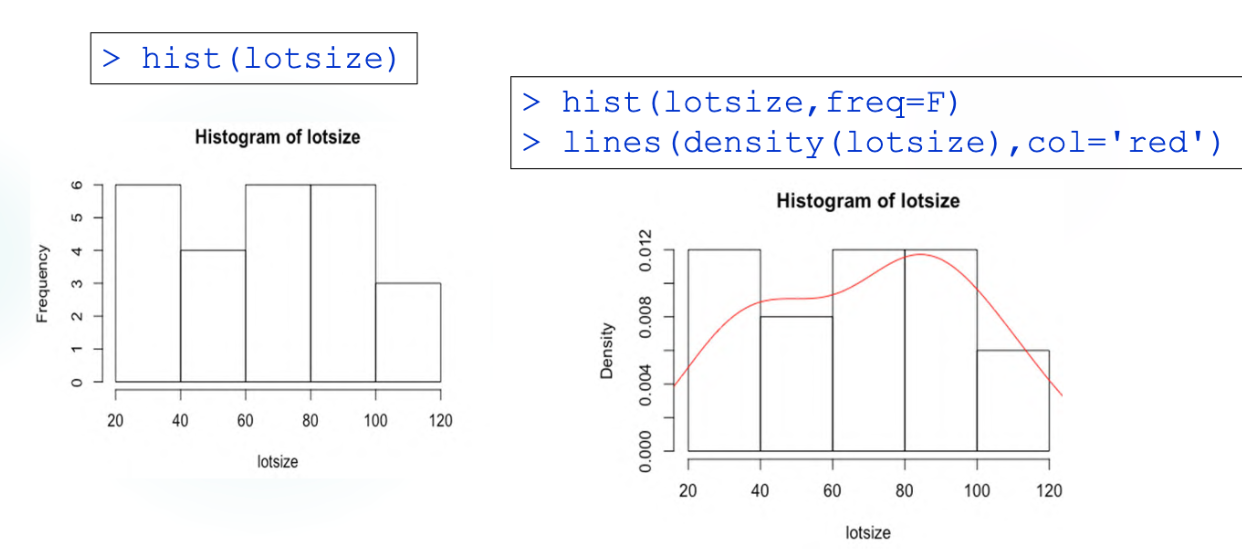
Quantile-Quantile Plots

Theory

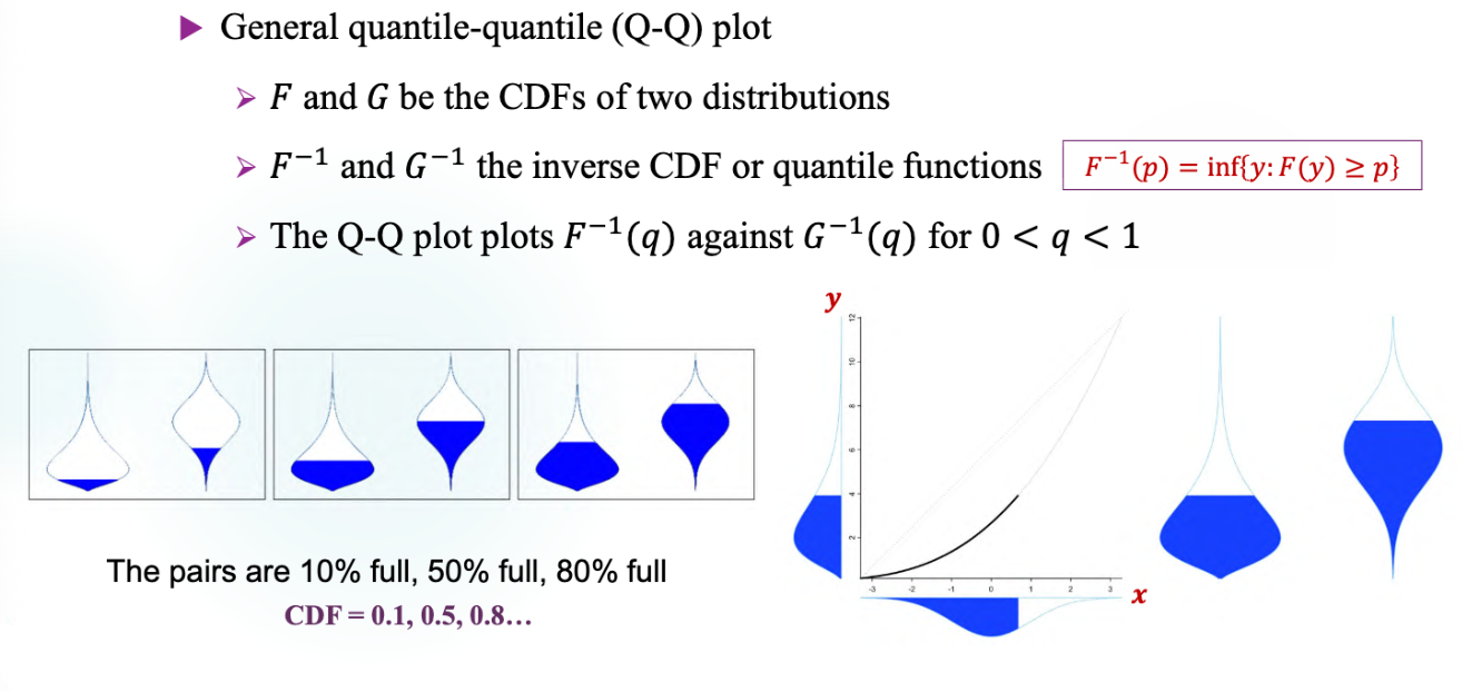
So the curve is not just in the first quadrant. The curve should be expressed as parametric equation:

$$\begin{cases} x(t)=F^{-1}(t) \\ y(t)=G^{-1}(t) \end{cases}, \ t\in [0,1]$$

Let's see normal quantile plots now.

Sample: $X_{1},\dots,X_{n}$. Then we have the empirical CDF

$$\hat{F}(x)=\frac{1}{n}\sum_{i=1}^{n}\mathbb{1}_{\{X_{i}\leq x\}}$$

, and can use this to plot the QQ plot against $\Phi^{-1}(x)$.

But in practice, the empirical CDF is a step function, so the curve would be stair-like, too. So actually we only plot some points on the plot. A common convention is to take

$$p_{i}=\frac{i-0.5}{n}$$

, which corresponds to the midpoint of each step of the empirical quantile function, and plot $(\Phi^{-1}(p_{i}),\hat{F}^{-1}(p_{i}))$.

So if the samples are from a normal distribution, then there should be

$$\hat{F}^{-1}(x)\approx \sigma\cdot\Phi^{-1}(x)+\mu$$

which is saying that the points should approximately scatter around a straight line.

Applications

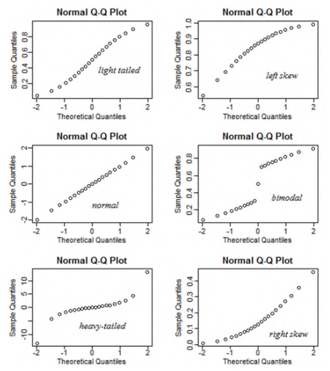
Taking the heavy-tailed one as an example for interpretation:

• when $p$ goes large, $\Phi^{-1}(p)$ hardly move but $\hat{F}^{-1}(p)$ moves a lot $\to$ there is plenty of density in the right side of the PDF $\to$ the right tail is heavy.
• same about the left tail.

Diagnostics Concerning the Residuals

Is the Relationship Linear?

• Plot $Y_{i}$ vs $X_{i}$
• Plot $e_{i}$ vs $X_{i}$ or $Y_{i}$ (residual plot)

Residual plots are better at emphasizing deviations from linear pattern.

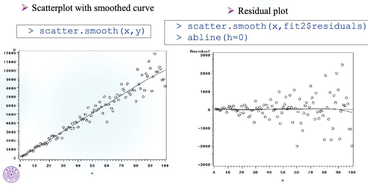
Example:

Run $Y\sim X$ to get the residuals and plot:

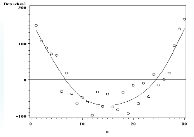
Quadratic pattern because $X^{2}$ is included in the residuals. $e_{i}$'s are delegating the non-linear part of $X_{i}^{2}$'s plus $\varepsilon_{i}$'s.

Does the Variance Differ across $X$ ?

By Plotting

• Plot $Y_{i}$ vs $X_{i}$
• Plot $e_{i}$ vs $X_{i}$ or $\hat{Y}_{i}$

Plot of $e_{i}$ vs $X_{i}$ will emphasize problems with the variance assumption.

Example:

The real model is

$$Y=30+100X+10X\varepsilon$$

Formal Test

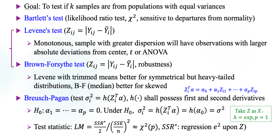
Let's take a look at the statistic in Breusch-Pagan test:

If the error variance depends on $X$, then $X$ can explain variations in the squared residuals $e_{i}^{2}$. As a result, $SSR^{*}$ tends to be large, leading to a larger LM statistic and making rejection of $H_{0}$ more likely.

The denominator does not necessarily differ systematically between $H_{0}$ and $H_{a}$. Its purpose is to standardize $SSR^{*}/2$ by the squared variance of errors under $H_{0}$, which equals to $\sigma^{4}$ under normality.

Assessment of Normality

Eye Tests

Common to use eye-test:

• Scatter in residual plot
• Box plot
• Histogram
• Normal quantile plot.

Correlation test can be used to make the test with normal quantile plot formal.

Formal Tests

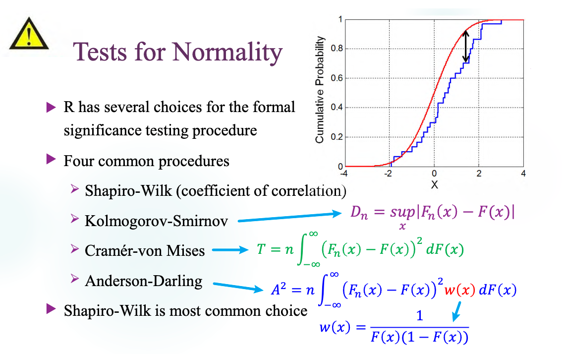
The principle of the Shapiro-Wilk test is similar to that of a Q-Q plot. Both assess how closely the observed quantiles align with the theoretical quantiles of a normal distribution.

Are Errors Dependent?

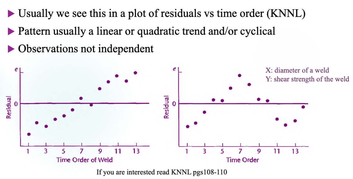
It seems that the order matters. We have to know the order though.

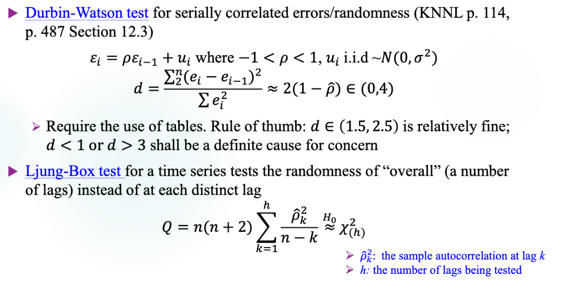
• DW tests first-order autocorrelation.
• LB tests multi-order autocorrelation.

Outliers

Model estimates based on means and sums of squares which are not robust to outliers.

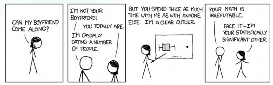
Significant other: a gender-neutral term for an intimate partner in a romantic relationship

Plot of $e_{i}$ vs $X_{i}$ should emphasize on outliers.

Here are two examples:

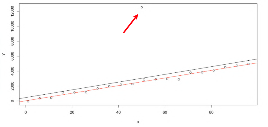
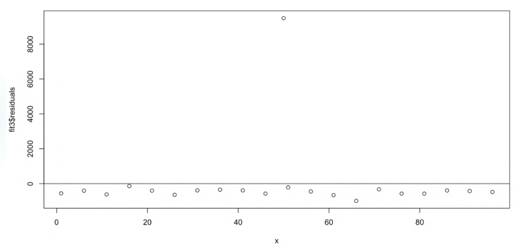
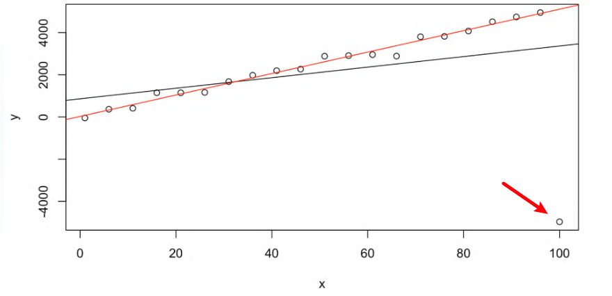
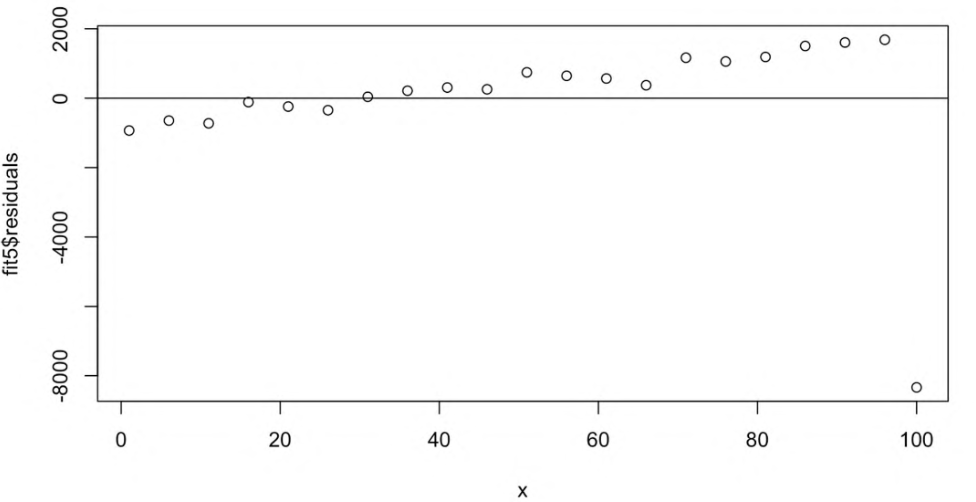
We can find that:

• Close to the mean $\to$ intercept influenced more
• Far from the mean $\to$ slope influenced more

However, both cases have larger $MSE$, which makes the p-value larger and the CIs wider. That is not what we want.

---

▶

notes on class

• 三阶矩，偏度，对称性
• 四阶矩，峰度，“-3”因为正态分布的前半部分算出来是3，尾部厚度，
  • super-gaussian：厚尾
  • sub-gaussian：薄尾
• 茎叶图，找众数
• 箱线图
• 直方图
• QQ 图，祖暅原理
• 诊断残差
  • 残差图
• 诊断同方差
  • Bartlett's test，似然比检验，依赖正态性假设
  • Levene's test
  • Brown-Forsythe test，Levene's modification，mean -> median
  • Breusch-Pagan test
• 诊断正态性
  • qq 图相关性检验
  • 统计学基本定理 经验 cdf - 理论 cdf 上确界为零 Glivenko–Cantelli Theorem
  • Shapiro-Wilk Test 依赖样本量
• 相关性检验，依赖更多信息，比如数据获取的顺序
  • Durbin-Watson test，检验一阶自相关
  • Ljung-Box test，检验多阶自相关
• Outlier，靠近均值，对斜率影响大