Fisher, Neyman, Reg 三种方法都是非参方法:不需要模型假设。共性:填补,以应对核心挑战。
有了模型假设,τ 就是模型参数的函数,我们应该估计参数并对参数估计量做推断。频率方法推导困难,贝叶斯方法更普适。贝叶斯框架中,参数天然就有分布。
搭建基础的分析框架很重要
Slides.
Motivation
Background:
- A random sample from a super population
- CRE
Goal
- Finite sample ACE (Average Causal Effect).
- Super population ACE.
Let's switch our point of view:
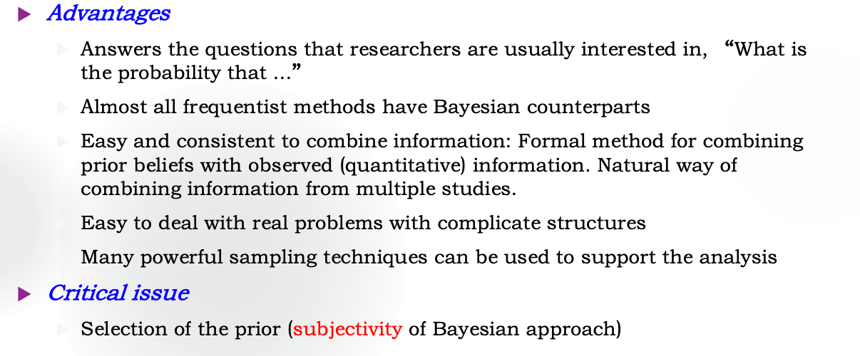
If we know the distribution of Y(1) and Y(0), then the ATE we concern is just a function of the parameters of the distribution. All we need to do is to estimate the parameters and conduct inference about them. So we introduce model-based methods here.
Bayesian Framework
Key opinion: treat unknowns (model parameters θ) as random variables.
Maybe the parameter is fixed in fact. But we don't know it. We are uncertain about it. We describe our uncertainty by treat the parameter as a random variable.
Main elements:
- Prior distribution p(θ).
- Likelihood function p(data∣θ).
- Joint distribution p(data,θ).
- Posterior distribution p(θ∣data).
Bayesian Model-Based Imputation
Finite Sample
Theory
Suppose we know the distribution of
- W∣Y(1),Y(0).
- (Y(1),Y(0))∣θ.
- θ.
Note that they are all joint distribution. If i.i.d., marginal distribution is enough.
With Yobs,W at hand, we can infer Ymiss by f(Ymiss∣Yobs,W). Then use them to estimate the finite sample ATE
τ=τ(Y(1),Y(0))=h(Ymis,Yobs,W).
That is, we want to know τ∣Yobs,W. The randomness comes from Ymis.
So we need to deduce
f(Ymiss∣Yobs,W)
θ is the bridge. See Yobs,W as pendants and we get
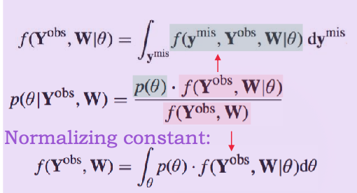
f(Ymiss∣Yobs,W)=∫θf(Ymiss∣Yobs,W,θ)p(θ∣Yobs,W)dθ
So we need f(Ymiss∣Yobs,W,θ) and p(θ∣Yobs,W).
Easy to deduce f(Ymis,Yobs∣W,θ) because given W, (Ymis,Yobs) is a linear combination of (Y(1),Y(0)).
And f(Ymis,Yobs,W∣θ) can be known because it is the multiplication of P(W∣θ) and f(Ymis,Yobs∣W,θ). The former one is known because CRE.

An Example
Read the slides from page 38 to 47. The results are the same as imputation with the mean of the observed value 😂.
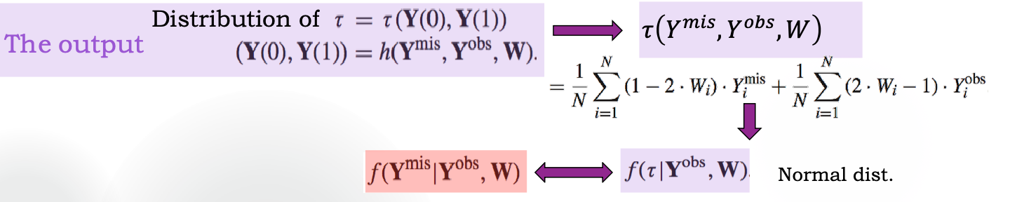
But the gain is that we know the distribution of τ∣Yobs,W, which allows us to easily conduct inference.
See Homework 3 where there are details.
Simulation
Challenges in Bayesian Inference:
- computation of the posterior distribution p(θ∣data).
- computation of the posterior predictive distribution p(y~∣y).
They are usually impossible to compute analytically in close form.
We can repeat:
- Impute θ.
- Impute Ymis.
- Calculate τ.
Then we can get a distribution of τ.
In View of Super Population
τsp=E[Yi(1)−Yi(0)]=τ(θ)
Note that τsp is also a random variable because of θ.
We want to know f(θ∣Yobs,W), which equals to
f(Yobs,W)p(θ)f(Yobs,W∣θ)
We can know the numerator, and the denominator is an integration of the numerator.
An analytic example:
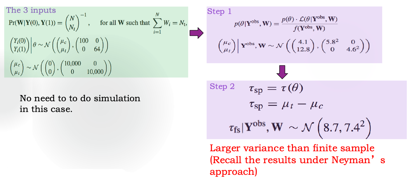
See Homework 3 for more detail.