4 Prediction and ANOVA

Slides.

yyy">Estimation and Prediction about $Y$

Estimation of $\mathbb{E}[Y_h]$

At $X=X_{h}$ the mean response is $\mathbb{E}[Y_h]=\beta_{0}+\beta_{1}X_{h}$. We estimate it with

$$\hat{\mu}_{h}=b_{0}+b_{1}X_h$$

Something about $\hat{\mu}_{h}:$

• Mean: Unbiased
• Variance: $\mathrm{Cov}(\bar{Y},b_1)=0$ is the key

$$\sigma^{2}(\hat{\mu}_{h})=\sigma^{2}\left[ \frac{1}{n}+ \frac{(X_{h}-\bar{X})^{2}}{S_{x x}} \right]$$

• Under i.i.d. normal error terms $\hat{\mu}_{h}\sim N(\mu_{h},\sigma^{2}(\hat{\mu}))$.
• $\dfrac{\hat{\mu}_{h}-{\mu}_{h}}{s(\hat{\mu}_{h})}\sim t_{n-2}$.

Note that the closer $X_{h}$ is to $\bar{X}$, the more precise $\hat{\mu}_{h}$ is. That why we say 线性回归适合做内差而不是外推。

Based on this significance tests and CIs can be obtained. For example, $100(1-\alpha)\%$ CI is

$$\hat{\mu}_{h}\pm t_{n-2,1-\alpha/2}s(\hat{\mu}_{h}).$$

Prediction of $Y_{h}$

Model:

$$Y_{h}=\beta_{0}+\beta_{1}X_{h}+\varepsilon$$

where $\varepsilon$ is not any one among $\varepsilon_{1},\dots,\varepsilon_N$, but has the same property, say uncorrelated and having the same variance.

We still use $\hat{\mu}_{h}$ to predict it. Here we need to consider $\varepsilon$. Let

$$d_{h}=Y_{h}-\hat{\mu}_{h}$$

we have

• Mean: $\mathbb{E}d_{h}=0$.
• Variance: The key is that $\varepsilon\perp (\varepsilon_{1},\dots,\varepsilon_{n})$.

$$\begin{align} \sigma^{2}(d_{h}) & = \mathbb{V}[(\beta_{0}-b_{0})+(\beta_{1}-b_{1})X_{h}{\color{red}+\varepsilon}] \\ & = \sigma^{2}\left[ {\color{red}1+}\frac{1}{n}+ \frac{(X_{h}-\bar{X})^{2}}{S_{x x}} \right] \end{align}$$

• Under normal error terms

$$d_{h}\sim N(0,\sigma^{2}(d_{h}))$$

• $\dfrac{d_{h}}{s(d_{h})}\sim t_{n-2}$.

The prediction intervals rely more on the normality assumption because $\varepsilon$ is alone. There is no average to allow CLT to perform.

Mean of $m$ New Observations

We still use $\hat{\mu}_{h}$ as the estimator. Let

$$d= \frac{1}{m}\sum_{i=1}^{m} Y_i^{new}-\hat{\mu}_{h}$$

Similarly

$$\sigma^{2}(d)=\dots=\sigma^{2}\left[ {\color{red}\frac{1}{m}}+\frac{1}{n}\frac{(X_{h}-\bar{X})^{2}}{S_{x x}} \right]$$

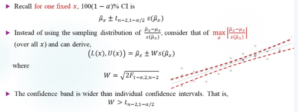
Confidence Band

If $L(x),U(x)$ (sample-dependent) satisfy

$$P[L(x)<\beta_{0}+\beta_{1}x<U(x)\ \forall x]=1-\alpha$$

Then the $100(1-\alpha)\%$ confidence band for the entire regression line is

$$\left\{ (x,y):L(x)<y<U(x), x \in \mathbb{R} \right\}$$

Note that we cannot just use the pointwise CIs to construct the confidence band. That is

$$\forall x, P[L(x)<\beta_{0}+\beta_{1}x<U(x)]=1-\alpha$$

Note that the "$\forall$" changes place. It is a bit similar to the difference between single inference and joint inference.

Summary

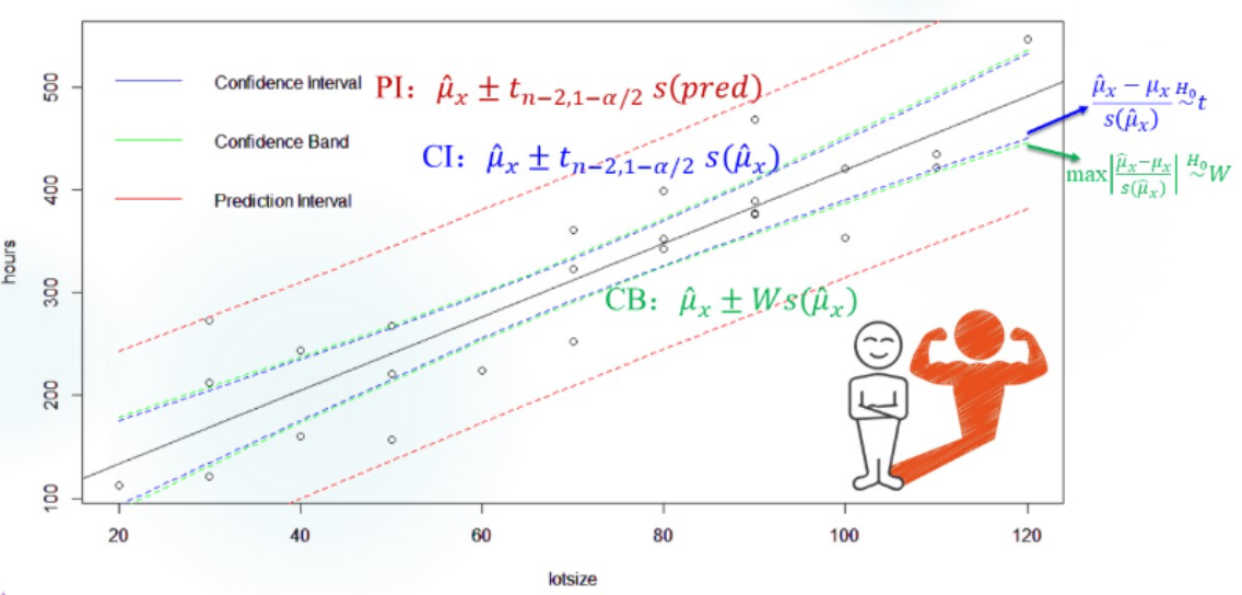
Prediction intervals are the widest. Confidence band is a little wider than CIs.

ANOVA

ANalysis Of VAriance.

Decomposition of Variation

$$\sum(Y_{i}-\bar{Y})^{2}=\sum (\hat{Y}_{i}-\bar{Y})^{2}+\sum (Y_{i}-\hat{Y}_{i})^{2}$$

which is

$$SST = SSR + SSE$$

• T: Total
• R: Regression
• E: Error
• It can be interpreted as an orthogonal decomposition

In some literature, R stands for residual and E stands for explained. In that sense, the meaning is completely different.

Let's see their degrees of freedom:

• SST: $n-1$, easy to understand
• SSR: $1$. It's because $SSR=b_{1}^{2}S_{x x}$. It's defined by $b_{1}$.
• SSE: $n-2$.

$MST,MSR,MSE$ are defined by $SST,SSR.SSE$ divided by their dfs.

---

As for the expectations, $SST$ and $SSE$ are easier to compute.

$$\begin{align} \mathbb{E}(Y_{i}-\bar{Y})^{2} & = \mathbb{E}(\beta_{1}(X_{i}-\bar{X})+\varepsilon_{i}-\bar{\varepsilon})^{2} \\ & = \beta_{1}^{2}(X_i-\bar{X})^{2}+ \frac{n-1}{n}\sigma^{2} \\ \implies \mathbb{E}(SST)& = \beta_{1}^{2}S_{x x}+ (n-1)\sigma^{2} \end{align}$$

And

$$\mathbb{E}(SSE)=(n-2)\sigma^{2}$$

So

$$\mathbb{E}(SSR)=\beta_{1}^{2}S_{x x}+\sigma^{2}$$

Expected Mean Squares

$$\begin{align} \mathbb{E}[MSR] & =\sigma^{2}+\beta_{1}^{2}S_{x x} \\ \mathbb{E}[MSE] & =\sigma^{2} \end{align}$$

When $\beta_{1}=0$, they equals to each other.

Let's Have a Deeper Look at DF

The model

$$Y=X\beta+\varepsilon$$

Suppose $\mathrm{rank}(X)=k$, full column rank. Then the projection matrix of $X$

$$P=X(X^TX)^{-1}X^T$$

has the same rank as $X$. Note that $\hat{Y}=PY$. So

$$SSE=\|\hat{Y}-Y\|^{2}=\|(P-I)Y\|^{2}$$

has df of $n-k$, because $\mathrm{rank}(P-I)=n-k$.

$$SST = \| Y-\frac{1}{n} \boldsymbol{1}\boldsymbol{1}^TY \|^{2}=\|(I-\frac{1}{n} \boldsymbol{1}\boldsymbol{1}^T)Y\|^{2}$$

has df of $n-1$ because $\mathrm{rank}(I-\frac{1}{n} \boldsymbol{1}\boldsymbol{1}^T)=n-1$.

$\frac{1}{n} \boldsymbol{1}\boldsymbol{1}^T$ is the projection matrix of $\boldsymbol{1}$.

$$SSR=\dots=\|(P-\frac{1}{n} \boldsymbol{1}\boldsymbol{1}^T)Y\|^{2}$$

has df of $k-1$ because $\mathrm{rank}(P-\frac{1}{n} \boldsymbol{1}\boldsymbol{1}^T)=k-1$.

Let $J=\frac{1}{n} \boldsymbol{1}\boldsymbol{1}^T$. Then $J$ is the projection matrix of a subspace of $\mathcal{R}(P)$. So $\mathcal R(P)$ can continue to be divided into two orthogonal subspaces:

$$\mathcal{R}(P)=\mathcal{R}(P-J)\oplus\mathcal{R}(J)$$

Therefore $\mathrm{rank}(P)=\mathrm{rank}(P-J)+\mathrm{rank}(J)$.

---

Moreover, $SST=SSR+SSE$ because

$$P-J \perp I-P$$

(It is easy to verify -- the multiplication is $O$.)

All thing above can be put in a nutshell:

$$\begin{align} Y & ={\color{blue}PY}+(I-P)Y \\ & = {\color{blue}(P-J)Y+JY}+(I-P)Y \end{align}$$

Subsequent orthogonal decomposition. In this note we will show that $(I-P)Y$ can continue to be orthogonally decomposed.

F-test

$$H_0: \beta_{1}\ne 0$$

When this holds, MSR tends to be larger than MSE. And because they all follow chi-square distribution and they are independent, we can set

$$F=\frac{MSR}{MSE}\sim F_{df_{R},df_{E}}$$

as the test statistic. When it's large enough, we can reject $H_0$ according to our significance level.

General Linear Test

A different view of the simple F-test.

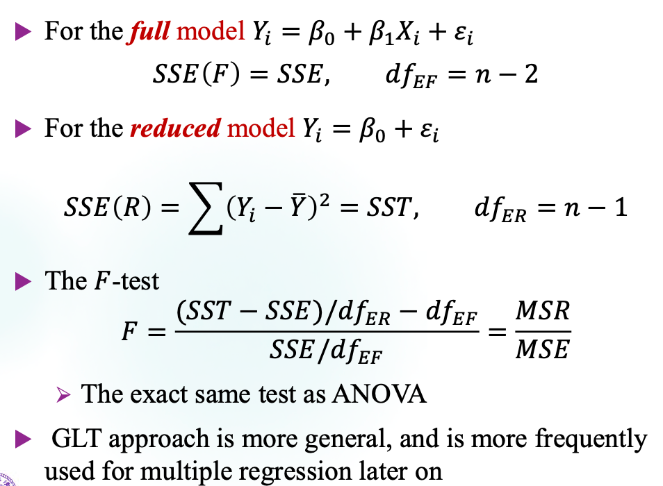
The principle is to compare the SSE of each model. The full model should have less SSE because we hope it can do better. More generally, the F-statistic should be written as

$$\frac{[SSE(R)-SSE(F)]/(df_{ER}-df_{EF})}{SSE(F)/df_{EF}}$$