2 Fisher's Exact P-Value and Neyman Repeated Sampling Approach

The slides are 2_FEP & Neyman Repeated Sampling Approach_handout_2026

Fisher's Exact P-Values

WHETHER THERE EXISTS A NON-ZERO UNIT-LEVEL CAUSAL EFFECT?

The Principles

Keep in mind that we want to study the causal effects. Conducting hypothesis testing is a good way to do that.

The basic steps of hypothesis testing:

1. State the hypothesis
2. Choose a test statistic
   • Its distribution should be known when $H_{0}$ holds
   • We should be able to calculate it with data at hand
3. Find the p-value
4. Compare with the given significance level

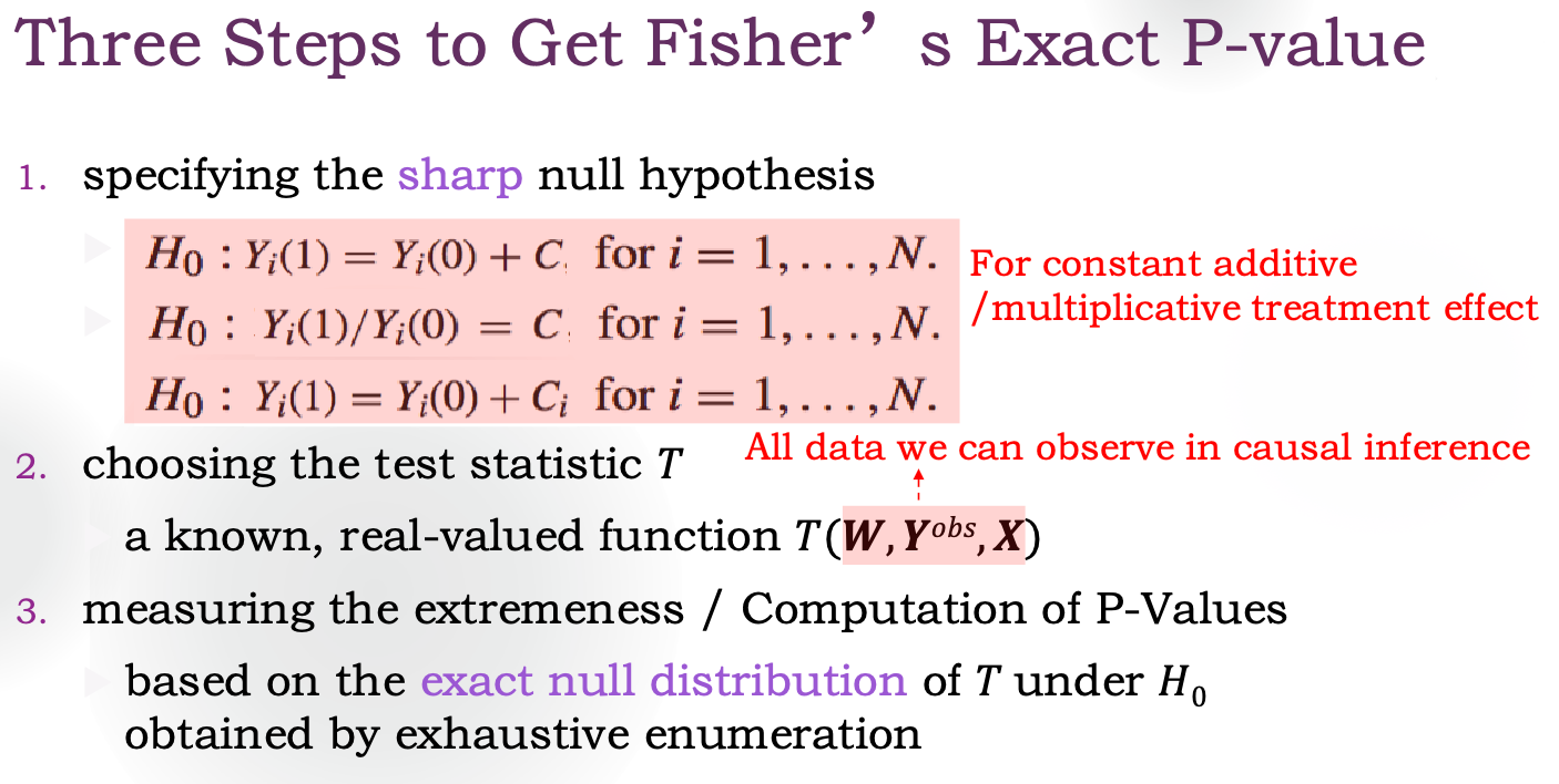
How to deal with the missing value problem? Fisher gave a solution: Fisher's sharp null hypothesis. It says:

$$H_{0}: Y_{i}(0) = Y_{i}(0)\quad \forall i$$

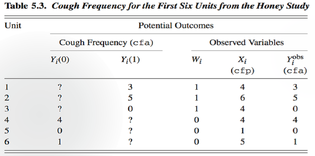
With $H_{0}$, we can fill in all the missing potential outcomes.

Select the following as the test statistic:

$$T^{\mathrm{dif}}=\bar{Y}_{t}^{obs}-\bar{Y}_{c}^{obs}$$

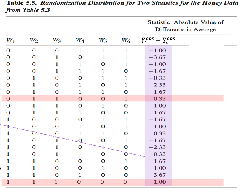
Note that the randomness in the r.v. comes from assignment. See this.

The next step is to find the null distribution of it. We enumerate all possible values of $\boldsymbol{W}$.

In this case, we got 1.00. Recall the definition of the p-value: the probability of the outcome being as extreme as or more extreme than the observed. Under this setting, we see $\geq 1.00$ and $\leq -1.00$ as extreme. Then the p-value is $\frac{16}{20}=0.8$.

Here is the summary slide. Note that

1. We can make various null hypothesis as long as long we can fill in the missing values with them.
2. All data we can observe can be used to construct the test statistic.

In Practice

Choosing the Test Statistic

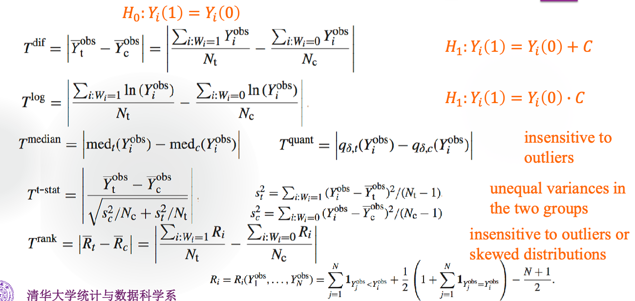
Many test statistics are proposed during class:

• $t:$ treatment, $c:$ control
• $N:$ the total number of the units in this experiment
• $N_{c}$: the number of units in control group

How to choose them? Recall that

$$\mathrm{Power}=P(\mathrm{reject}\ H_{0}\mid H_{0} \text{ is false})$$

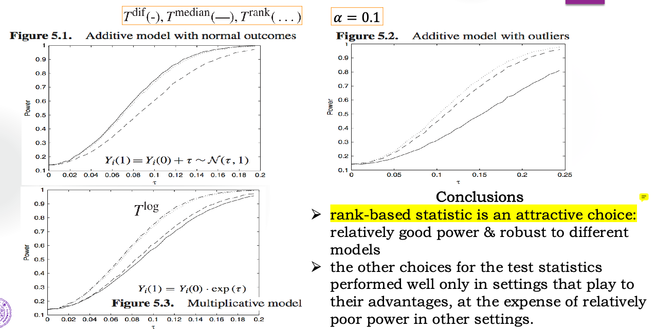
In the following figures, $\tau$ means the real causal effect. So the point where $\tau=0$ says the probability of the type I error, thus all of the three statistics are valid. But their effectiveness is different.

Computation of P-Values

Computing exact p-value is very expensive when $N_{c}, N_{t}$ are both large. Two methods to approximate it were proposed during class:

Approximate P-Value by Simulation

• randomly choose a subset of $K$ possible assignment vectors
• For each assignment vector obtained, calculate its test statistics

$$T^{\mathrm{dif},k} = \bar{Y}_{t,k}-\bar{Y}_{c,k}$$

• approximate the p-value by

$$\hat{p}=\frac{1}{K}\sum_{k=1}^{K} \mathbb{1}_{T^{\mathrm{dif},k}\geq T^{\mathrm{dif},obs}}$$

The math behind it is:

Suppose there are $N$ possible assignment vectors, and their corresponding $T^{\mathrm{dif}}$'s are $x_1,\dots,x_N$, and our observed one is $x_n$. The real p-value is

$$p = \frac{\# \left\{ i: x_i\geq x_n \right\}}{N}$$

Let

$$X_k=\begin{cases} 1, & \text{if } T^{\mathrm{dif},k}\geq T^{\mathrm{dif,obs}} \\ 0, & \text{o.w.} \end{cases}$$

Then $X_k$'s are i.i.d. Bernoulli r.v.s with parameter $p$. According to the CLT

$$\frac{\bar{X}-p}{\sqrt{p(1-p)/K}} \overset{d}{\to}N(0,1)$$

Note that the s.e. has an upper bound of $1/2\sqrt{K}$

Approximate P-Value by Two-Sample T-Test

First introduce the Finite Population CLT:

Suppose the population is $x_1,\dots,x_N$, the population mean and population variance are

$$\bar{x}=\frac{1}{N}\sum x_i\quad S^{2}=\frac{1}{N-1}\sum(x_i-\bar{x})^{2}$$

if we do random sampling without replacement with sample size $n$ (it's equivalent to assign a random $\boldsymbol{W}$), and get sample mean $\bar{x}_{\mathrm{sample}}$. Then we have

$$\mathbb{E}(\bar{x}_{\mathrm{sample}})=\bar{x}\quad \mathrm{Var}(\bar{x}_{\mathrm{sample}})=\left( 1-\frac{n}{N} \right) \frac{S^{2}}{n}$$

the derivation of the variance is similar to ^the-transformation.
And when $N\to \infty$, if $\frac{n}{N}\to a\in(0,1)$ and no outlier in the population, we have

$$\frac{\bar{x}_{\mathrm{sample}}-\bar{x}}{\sqrt{\mathrm{Var}(\bar{x}_{\mathrm{sample}})}}\overset{d}{\to}N(0,1)$$

Note that is origin of randomness in $\bar{x}_\mathrm{sample}$ is the same as $\bar{Y}_{t}^{obs}-\bar{Y}_{c}^{obs}$: the assignment $\boldsymbol{W}$. And the structures of them are similar, so $\bar{Y}_{t}^{obs}-\bar{Y}_{c}^{obs}$ also has the approximate normality.

Under $H_0$ we have

$$\begin{align} \mathbb{E}[\bar{Y}_{t}^{obs}-\bar{Y}_{c}^{obs}] & =0 \\ \mathbb{V}[\bar{Y}_{t}^{obs}-\bar{Y}_{c}^{obs}] & =\frac{N}{N_tN_c}S^{2} \end{align}$$

where $S^{2}=\frac{1}{N-1}\sum_{i=1}^{N}\left( Y_i(1)-\bar{Y}(1) \right)^{2}=\frac{1}{N-1}\sum_{i=1}^{N}\left( Y_i(0)-\bar{Y}(0) \right)^{2}$

According to the finite population CLT, under $H_0$ we have

$$\frac{\bar{Y}_{t}^{obs}-\bar{Y}_{c}^{obs}}{\sqrt{\frac{N}{N_tN_c}S^{2}}}\overset{d}{\to} N(0,1)$$

Replace $S^2$ with pooled sample variance

$$s^{2}=\frac{1}{N-2}\left[ \sum_{i:W_i=1}\left( Y_i(1)-\bar{Y}^{obs}_t \right)^{2}+\sum_{i:W_i=0}\left( Y_i(0)-\bar{Y}^{obs}_c \right)^{2} \right]$$

we still have

$$\frac{\bar{Y}_{t}^{obs}-\bar{Y}_{c}^{obs}}{\sqrt{\frac{N}{N_tN_c}s^{2}}}\overset{d}{\to} N(0,1)$$

(the path to this conclusion is already paved by mathematicians (Slutsky), we just go through it)

So we can just do a two-sample t-test assuming equal variance on the data and get the p-value which can be used to approximate the p-value desired.

On the other hand, we can also replace $S^{2}$ with $\frac{1}{N_{t}}s_{t}^{2}+\frac{1}{N_{c}}s_{c}^{2}$ (see A Special Case), and

$$\frac{\bar{Y}_{t}^{obs}-\bar{Y}_{c}^{obs}}{\sqrt{\frac{s_{t}^{2}}{N_{t}}+\frac{s_{c}^{2}}{N_{c}}}}\overset{d}{\to} N(0,1)$$

also holds, which means we can also use the p-value from two-sample t-test without assuming equal variance to approximate the p-value desired.

Neyman's Repeated Sampling Approach

HOW TO ESTIMATE THE AVERAGE CAUSAL EFFECT?

Limitations of Fisher's method:

• The sharp null hypothesis is somewhat restrictive
• Rejecting the null hypothesis itself cannot provide us an estimator of the unknown (average) treatment effect

Neyman's approach:

• Focus on average causal effect instead of unit-level effect
• Provide unbiased point estimator & interval estimator
• Randomness: considering only finite population first
  • randomized assignment of treatments to the units in the sample

Estimation of ATE

Causal estimand (some value to be estimated):

$$\tau_{fs} = \frac{1}{N}\sum_{i=1}^{N} (Y_{i}(1)-Y_{i}(0)) = \bar{Y}(1)-\bar{Y}(0)$$

where

$$\bar{Y}(1)=\frac{1}{N}\sum_{i=1}^{N} Y_{i}(1),\quad \bar{Y}(0)=\frac{1}{N}\sum_{i=1}^{N} Y_{i}(0)$$

Our estimator is

$$\hat{\tau}^{\mathrm{dif}}=\bar{Y}^{obs}_{t}-\bar{Y}^{obs}_{c}$$

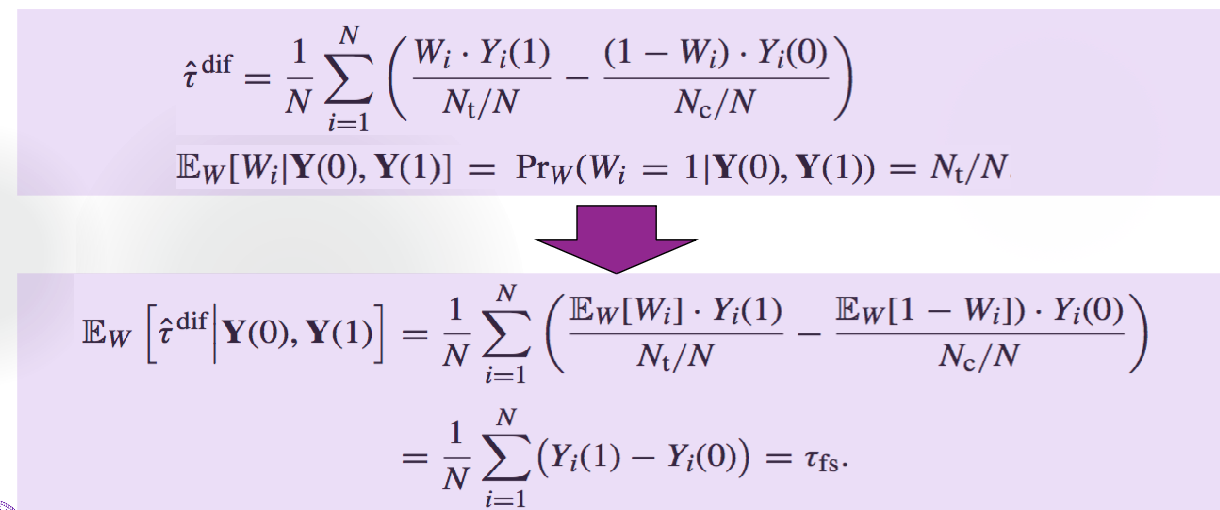
The estimator is unbiased:

Note that we are conditioning on $\boldsymbol{Y}(0),\boldsymbol{Y}(1)$. Wait, but they are not r.v.s, what is the meaning of conditioning on them?

Building Confidence Interval

3 steps:

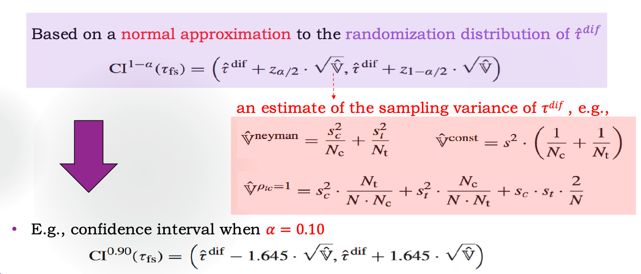
• Derive the sampling variance of the estimator
• Develop a estimator for the sampling variance
• Create a large-sample confidence interval

Variance Deriving

Let's derive the sampling variance of $\hat{\tau}^{\mathrm{dif}}$, first we separate parts with and without randomness:

$$\begin{align} \hat{\tau}^{\mathrm{dif}}&= \frac{1}{N_{t}}\sum_{i=1}^{N} W_{i}Y_{i}-\frac{1}{N_{c}}\sum_{i=1}^{N} (1-W_{i})Y_{i}\\ & = \frac{1}{N_t} \sum W_i Y_i(1) - \frac{1}{N_c} \sum (1-W_i) Y_i(0)\quad (\text{partialing out }Y_{i}\text{'s randomness}) \\ & =\sum \left[ \left(\frac{Y_i(1)}{N_t} + \frac{Y_i(0)}{N_c}\right) W_i - \frac{Y_i(0)}{N_c} \right] \\ & = \sum A_i W_i - \sum \frac{Y_i(0)}{N_c} \end{align}$$

Before we start computing the variance, we derive $\mathrm{Var}(W_{i})$ and $\mathrm{Cov}(W_{i},W_{j}),i\ne j$.

$$\begin{align} \mathrm{Var}(W_{i}) & = \frac{N_{t}}{N}\left( 1-\frac{N_{t}}{N} \right) \\ \mathrm{Cov}(W_{i},W_{j}) & = \mathbb{E}(W_{i}W_{j})-\mathbb{E}(W_{i})\mathbb{E}(W_{j}) \\ & = \frac{N_{t}}{N}\cdot \frac{N_{t}-1}{N-1}-\frac{N_{t}^{2}}{N^{2}} \end{align}$$

Next, compute the variance:

$$\begin{align} \mathrm{Var}\left( \sum A_{i}W_{i} \right) & = \sum A_i^2 \text{Var}(W_i) + \sum_{i \neq j} A_i A_j \text{Cov}(W_i, W_j) \\ & = \sum A_{i}^{2} \frac{N_{t}N_{c}}{N^{2}}-\sum_{i\ne j}A_{i}A_{j} \frac{N_{t}N_{c}}{N^{2}(N-1)} \\ & = \color{blue}\frac{N_t N_c}{N^2} \sum A_i^2 - \frac{N_t N_c}{N^2(N-1)} \left[ \left(\sum A_i\right)^2 - \sum A_i^2 \right] \\ & = \frac{N_t N_c}{N(N-1)} \left[ \sum A_i^2 - \frac{1}{N} (\sum A_i)^2 \right] \\ & = \frac{N_t N_c}{N(N-1)} \sum (A_i - \bar{A})^2\quad (!) \end{align}$$

Let

$$\begin{align} S_{c}^{2}&=\frac{1}{N-1}\sum_{i=1}^{N} \left( Y_{i}(0)-\bar{Y}(0) \right) ^{2} \\ S_{t}^{2}&=\frac{1}{N-1}\sum_{i=1}^{N} \left( Y_{i}(1)-\bar{Y}(1) \right) ^{2} \\ S_{tc}^{2} & = \frac{1}{N-1} \sum_{i=1}^{N} \left( Y_{i}(1)-Y_{i}(0)-(\bar{Y}(1)-\bar{Y}(0)) \right) ^{2} \\ C_{tc} & = \frac{1}{N-1}\sum_{i=1}^{N} \left(Y_{i}(0)-\bar{Y}(0)\right)\left(Y_{i}(1)-\bar{Y}(1)\right) \end{align}$$

Then we have

$$\frac{1}{N-1}\sum_{i=1}^{N} (A_{i}-\bar{A})^{2}=\frac{1}{N_{t}^{2}}S_{t}^{2}+\frac{1}{N_{c}^{2}}S_{c}^{2}+\frac{2}{N_{t}N_{c}}C_{tc}$$

Note that

$$S_{tc}^{2}=S_{t}^{2}+S_{c}^{2}-2C_{tc}$$

Plug it in, we get

$$\mathrm{Var}(\hat{\tau}^{\mathrm{dif}})=\frac{1}{N_{t}}S_{t}^{2}+\frac{1}{N_{c}}S_{c}^{2}-\frac{1}{N}S_{tc}^{2}$$

A Special Case

If $Y_{i}(1)-Y_{i}(0)= \bar{Y}(1)-\bar{Y}(0) = \tau_{fs},\ \forall i$, then we have $S_{tc}^{2}=0$, and thus

$$\mathrm{Var}(\hat{\tau}^{\mathrm{dif}})=\mathbb{V}^{\mathrm{const}}=\frac{1}{N_{t}}S_{t}^{2}+\frac{1}{N_{c}}S_{c}^{2}$$

Alternative Representation

Let

$$\rho_{tc}=\frac{C_{tc}}{S_{t}S_{c}}$$

then

$$\mathrm{Var}(\hat{\tau}^{\mathrm{dif}})=\frac{N_{t}}{N N_{c}}S_{c}^{2}+\frac{N_c}{N N_{t}}S_{t}^{2}+\frac{2}{N}\rho_{tc}S_{c}S_{t}$$

Variance Estimating

Based on the two representations of $\mathrm{Var}(\hat{\tau}^{\mathrm{dif}})$, two conservative estimators are proposed:

$$\begin{align} \hat{\mathbb{V}}^{\mathrm{neyman}} & = \frac{s_{c}^{2}}{N_{c}}+\frac{s_{t}^{2}}{N_{t}} \\ \hat{\mathbb{V}}^{\rho_{tc}=1}&=s_c^{2}\cdot \frac{N_t}{N\cdot N_c}+s_c^{2}\cdot \frac{N_c}{N\cdot N_t}+s_cs_t\cdot \frac{2}{N} \\ & =\frac{s_c^{2}}{N_c}+\frac{s_t^{2}}{N_t}-\frac{(s_t-s_c)^{2}}{N} \end{align}$$

where

$$\begin{align} s_{c}^{2}&=\frac{1}{N_{c}-1}\sum_{i:W_{i}=0}\left( Y_{i}^{\mathrm{obs}}-\bar{Y}_{c}^{\mathrm{obs}} \right)^{2} \\ s_{t}^{2}&=\frac{1}{N_{t}-1}\sum_{i:W_{i}=1}\left( Y_{i}^{\mathrm{obs}}-\bar{Y}_{t}^{\mathrm{obs}} \right)^{2} \\ \end{align}$$

$s_c^{2},s_t^{2}$ are unbiased estimators for $S_c^{2},S_t^{2}$ respectively.

Theorem If the treatment effect $Y_{i}(1)-Y_{i}(0)$ is constant, then an unbiased estimator for the sampling variance is

$$\hat{\mathbb{V}}^{\mathrm{neyman}}= \frac{s_{c}^{2}}{N_{c}}+\frac{s_{t}^{2}}{N_{t}}$$

If $S_{t}^{2}=S_c^{2}$,

$$\hat{\mathbb{V}}^{\mathrm{const}}=s^{2}\left( \frac{1}{N_c}+\frac{1}{N_t} \right)$$

where

$$s^{2}=\frac{1}{N-2}\left( s_c^{2}(N_c-1)+s_t^{2}(N_t-1) \right)$$

which is the weighted average of both variance estimators.

Confidence Intervals

We have discussed the approximate normality of $\hat{\tau}^{\mathrm{dif}}$ before. Replacing the real variance with a decent estimate doesn't break it.

Some Other Things

See CI-HW3 › Problem 3 (Treatment Effect Heterogeneity).

Super Population

Concepts

The finite units of size $N$ can be viewed as a random sample from an infinite super-population where $(X_i,Y_i(0),Y_i(1))$ are i.i.d. draws ($X_i$ is covariate).

Note that from now on $Y_{i}(0),Y_{i}(1)$ have had randomness. All conclusions above can be seen as conditional given all $(Y_{i}(0),Y_{i}(1))$'s. (Below I use $\mid Y$ to denote this.)

List some notations here:

$$\begin{align} \sigma^{2}_{c} & =\mathbb{V}[Y_{i}(0)] \\ \sigma^{2}_{t} & =\mathbb{V}[Y_{i}(1)] \\ \sigma^{2}_{tc} & = \mathbb{V}[Y_{i}(1)-Y_{i}(0)] \end{align}$$

We can show the expectations of $S^{2}_{c},S^{2}_{t},S^{2}_{tc}$ are $\sigma^{2}_{c},\sigma^{2}_{t},\sigma^{2}_{tc}$ respectively.

▶

Proof of S^2_c

$$\begin{align} \mathbb{E}[S^{2}_{c}] & = \mathbb{E}\left[ \frac{1}{N-1}\sum_{i=1}^{N} (Y_{i}(0)-\bar{Y}_{i}(0))^{2} \right] \end{align}$$

We just need to focus on $\mathbb{E}[(Y_{i}(0)-\bar Y_{i}(0))^{2}]$. Below let $Y_{i}=Y_{i}(0),\mu=\mathbb{E}(Y_{i}(0))$

$$\begin{align} \mathbb{E}[(Y_{i}(0)-\bar Y_{i}(0))^{2}] & = \color{blue} \mathbb{E}[(Y_{i}-\mu+\mu-\bar{Y})^{2}] \\ & = \mathbb{E}(Y_{i}-\mu)^{2}+\mathbb{E}(\bar{Y}-\mu)^{2}+2\mathbb{E}(Y_{i}-\mu)(\mu-\bar{Y}) \\ & = \mathbb{V}[Y_{i}]+\frac{1}{N}\mathbb{V}[Y_{i}]-\frac{2}{N}\mathbb{V}[Y_i] \\ & = \frac{N-1}{N}\sigma^{2}_{c} \end{align}$$

Deliberation on the cross term:

$$\begin{align} \mathbb{E}(Y_{i}-\mu)(\bar{Y}-\mu) & = \mathbb{E}\left[ (Y_i-\mu)\cdot \frac{1}{N}\sum_{k=1}^{N} (Y_k-\mu) \right] \\ & = \mathbb{E}\left[ \frac{1}{N}\sum_{k=1}^{N} (Y_k-\mu)(Y_i-\mu) \right] \\ & = \frac{1}{N}\sum_{k=1}^{N} \mathbb{E}(Y_k-\mu)(Y_i-\mu) \\ & = \frac{1}{N}\mathbb{V}[Y_{i}] \end{align}$$

or

$$\mathbb{E}(Y_{i}-\mu)(\bar{Y}-\mu)=\mathrm{Cov}(Y_i,\bar{Y})=\dots$$

Population ATE

The causal estimand for a super population:

$$\tau _{sp}=\mathbb{E}[Y_{i}(1)-Y_{i}(0)]$$

$\tau _{fs}$ is a proxy for $\tau _{sp}$.

$$\mathbb{E}[\tau _{fs}]=\mathbb{E}\left[ \frac{1}{N}\sum (Y_{i}(1)-Y_{i}(0))\right]=\tau _{sp}$$

$$\begin{align} \mathbb{V}[\tau _{fs}] & = \mathbb{V}[\dots] \\ & = \frac{1}{N^{2}}\sum_{i=1}^{N} \mathbb{V}[Y_{i}(1)-Y_{i}(0)] \\ &= \frac{\sigma^{2}_{tc}}{N} \end{align}$$

Inference for Population ATE

$\hat{\tau}^{\mathrm{dif}}$ is a proxy for $\tau _{fs}$, can it be used to understand the super population?

The answer is yes.

Note that the randomness in $\hat{\tau}^{\mathrm{dif}}$ now has two sources:

• Assignment $W_1,\dots,W_N$
• Sampled potential outcomes $Y_1(0),\dots,Y_N(0),Y_1(1),\dots,Y_N(1)$

There are different types of randomization of assignment, here I introduce two:

1. Bernoulli randomization: it says $W_i\overset{i.i.d.}{\sim}\mathrm{Bern}(p)$.
2. Complete randomization: it is to randomly choose $N_{t}$ out of $N$ units to receive treatment.

$$\mathbb{E}[\hat{\tau}^{\mathrm{dif}}]=\mathbb{E}_Y[\mathbb{E}_W[\hat{\tau}^{\mathrm{dif}}\mid Y]]=\mathbb{E}_Y[\tau _{fs}]=\tau _{sp}$$

For the variance

$$\begin{align} \mathbb{V}[\hat{\tau}^{\mathrm{dif}}] & = \mathbb{E}[(\hat{\tau}^{\mathrm{dif}}-\tau _{sp})^{2}] \\ & = \color{blue} \mathbb{E}[(\hat{\tau}^{\mathrm{dif}}-\tau _{fs}+\tau _{fs}-\tau _{sp})^{2}] \end{align}$$

Expanding it yields 3 components:

$$\begin{align} \mathbb{E} & [(\hat{\tau}^{\mathrm{dif}}-\tau _{fs})^{2}] \\ \mathbb{E} & [(\tau _{fs}-\tau _{sp})^{2}] \\ 2\mathbb{E} & (\hat{\tau}^{\mathrm{dif}}-\tau _{fs})(\tau _{fs}-\tau _{sp}) \end{align}$$

The first term

$$\begin{align} \mathbb{E}[(\hat{\tau}^{\mathrm{dif}}-\tau _{fs})^{2}] & = \mathbb{E}[\mathbb{E}[\dots\mid Y]]\\ \\ & = \mathbb{E}\left[ \frac{S^{2}_{c}}{N_c}+\frac{S^{2}_{t}}{N_t}-\frac{S^{2}_{tc}}{N} \right] \\ & = \frac{\sigma^{2}_{c}}{N_{c}}+\frac{\sigma^{2}_{t}}{N_{t}}-\frac{\sigma^{2}_{tc}}{N} \end{align}$$

The second term equals to $\mathbb{V}[\tau _{fs}]=\frac{\sigma^{2}_{tc}}{N}$. The third term equals to 0 because $\mathbb{E}[\hat{\tau}^{\mathrm{dif}}-\tau _{fs}\mid Y]=0$.

So

$$\mathbb{V}[\hat{\tau}^{\mathrm{dif}}]=\frac{\sigma^{2}_{c}}{N_{c}}+\frac{\sigma^{2}_{t}}{N_{t}}$$

Therefore

$$\frac{s^{2}_{c}}{N_c}+\frac{s^{2}_{t}}{N_t},$$

which is exactly the Neyman estimator $\hat{\mathbb{V}}^{\mathrm{neyman}}$, can be used to estimate the variance.