6 Remedies and Miscellaneous Topics

Slides.

More Diagnostics for Residuals

Review Residual Plots

Should do EDA first. Use

scatter.smooth(X,Y)

to get a smoothed curve fit to see the relation ship between $X$ and $Y$.

Let see some examples:

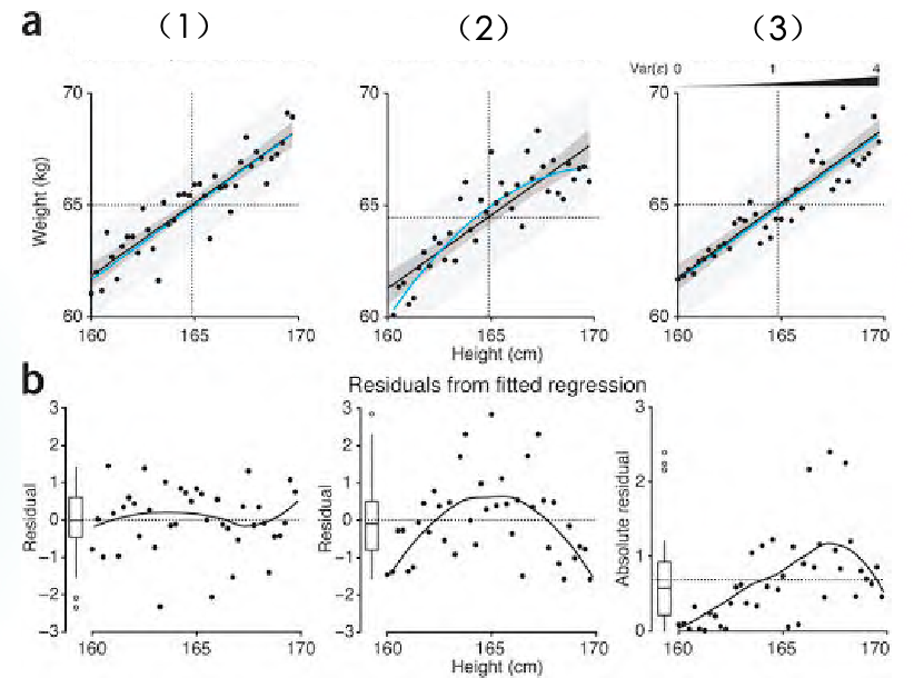
1. No obvious violation
2. Nonlinearity. Because at some $X$ the residuals are all negative or positive.
3. Non-constant variance. Note that the residual plot below uses absolute residual as the y-label, aiming to see the scale of residuals.

---

Built-in diagnostic plots in R

reg <- lm(hours ~ lotsize, data=toluca)
plot(reg)

R will show four diagnostic plots one by one:

1. Residuals vs Fitted
2. Normal Q-Q
3. Scale-Location
4. Residuals vs Leverage

Points with numbers next to them in each plot are extreme values. The numbers are the index of them, letting us to check the original data.

Residuals vs Fitted

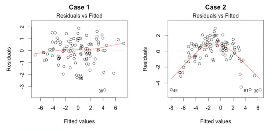
• Why $\hat{Y}$? To combine all explanatory variables' influences, easy to move to multiple linear regression.
• Used to check if the residuals have non-linear patterns.
• It’s good if residuals equally spread around a horizontal line without distinct patterns.

Normal Q-Q

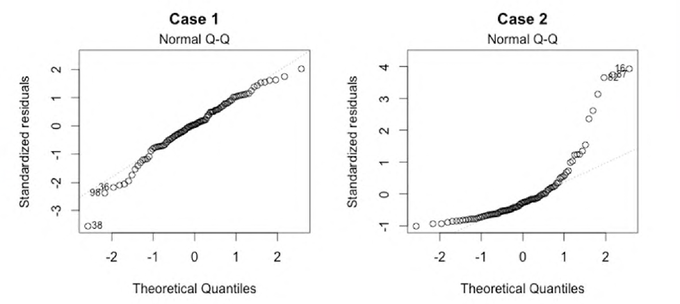
• Used to check if the residuals are normally distributed.
• It’s good if residuals are lined well on the straight dashed line.

Standardized residual is defined as

$$\frac{e_{i}}{s\sqrt{1-h_{ii}}}$$

where $h_{ii}= \frac{\partial \hat{Y}_{i}}{\partial Y_{i}}=\frac{1}{n}+ \frac{(X_{i}-\bar{X})^{2}}{S_{x x}}$, the leverage. It will be discussed in the next lecture.

Note that

$$\mathbb{V}[e_{i}\mid \boldsymbol{X}] = (1-h_{ii})\sigma^{2}$$

The reason why standardized residual is used is that $e_{i}$ are not i.i.d. so they cannot be directly used to delegate the real $\varepsilon_{i}$. Pre-process needed.

Scale-Location

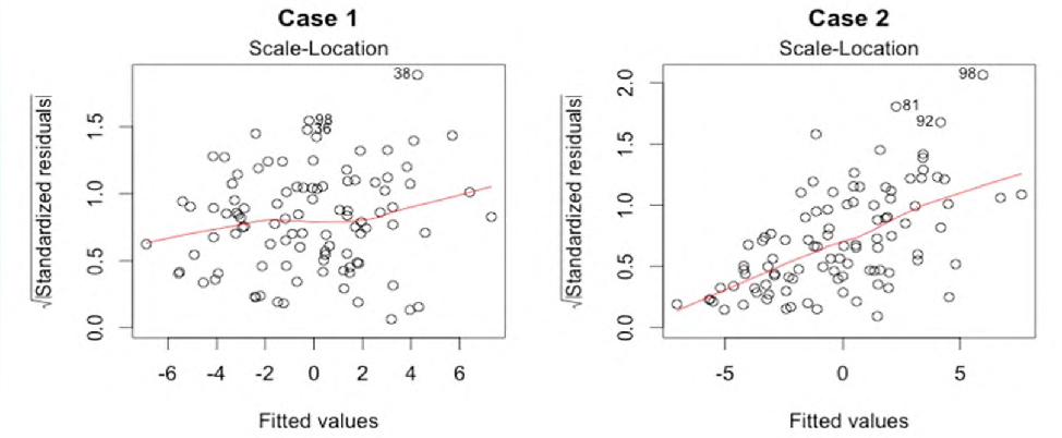
• It shows if residuals are spread equally along the ranges of predictors
• Check the assumption of equal variance (homoscedasticity)
• It’s good if you see a horizontal line with equally (randomly) spread points

Residuals vs Leverage

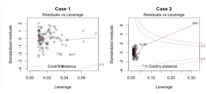
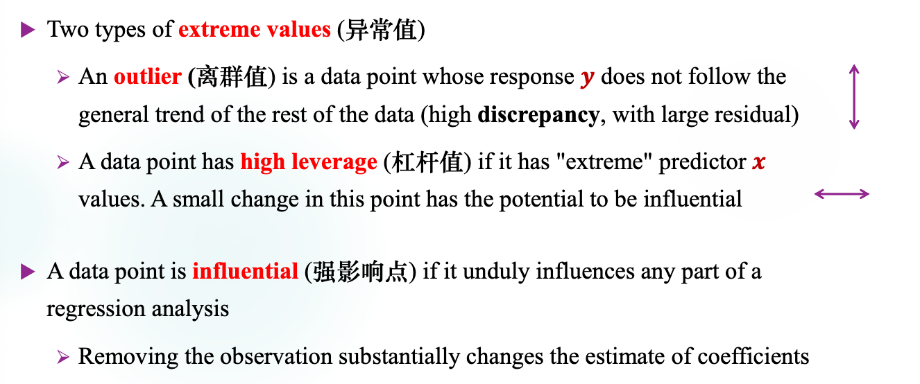
Leverage, also known as the observation self-sensitivity or self-influence

$$h_{ii}=\frac{\partial \hat{Y}_{i}}{\partial Y_{i}}=\frac{1}{n}+ \frac{(X_{i}-\bar{X})^{2}}{S_{x x}}\in [0,1]$$

For design matrix $X_{n\times p}$, $s^{2}=\frac{e^Te}{n-p}$. Cook's distance is defined as

$$D_{i}=\frac{\sum_{j=1}^{N} (\hat{Y}_{j}-\hat{Y}_{j(-i)})^{2}}{ps^{2}}=\frac{e_{i}^{2}}{ps^{2}}\cdot \frac{h_{ii}}{(1-h_{ii})^{2}}$$

where $\hat{Y}_{j(-i)}$ is the fitted response value obtained when excluding the $i$-th observation. It measures the influence of $i$-th case on all predicted values.

给定 $h_{ii}$ 和 $D_{i}$，可以解出标准化残差的平方，故可以画出两条对称的等值线。

F-Test for Lack of Fit

When we have repeat observations at various values of $X$, the error term will be partitioned into pure error (error within replicates) and a lack of fit error.

$$\begin{align} H_0 & : \text{There is no lack of fit in the regression model} \\ H_{1} & : \text{o.w.} \end{align}$$

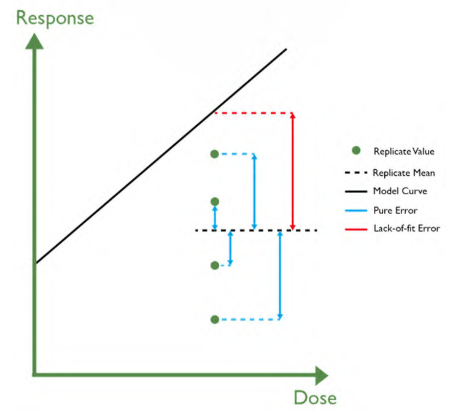
Use GLT, the basic idea is to compare two models -- the full one and the reduced one. Then here comes the question, what are the two models?

Suppose there are $c$ different observed values of $X_{i}$: $x_{1},\dots,x_{c}$. So there are $c$ groups, and within each group $i$, there are $n_{i}$ observations. Let $Y_{ij}$ be the $j$-th response in the $i$-th group.

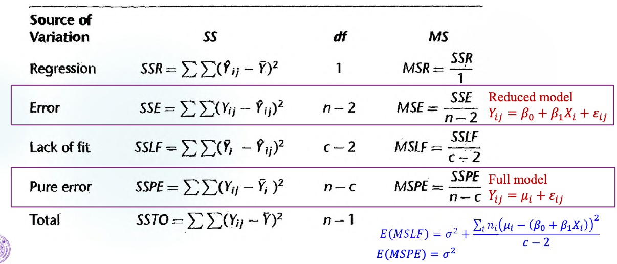
If $H_{0}$ holds, then the mean response $\mu_{i}=\beta_{0}+\beta_{1}X_{i}$. The reduced model is

$$Y_{ij}=\beta_{0}+\beta_{1}X_{i}+\varepsilon_{ij}$$

Run regression and get $SSE(R)$. Its df is $n-2$.

Suppose that $X_{i}$ can take $m$ values $x_{1},\dots,x_{m}$. Then the full model is

$$Y_{ij}=\mu_{i}+\varepsilon_{ij}$$

Run regression and get $SSE(F)=SSPE$ (Pure Error). Note that this model has as many parameters as the number of the groups. So its df is $n-c$.

And we can get

$$F=\frac{[SSE(R)-SSE(F)]/(df_{ER}-df_{EF})}{SSE(F)/df_{EF}}$$

There is a relationship

$$SSE=SSPE+SSLF$$

Let's Have a Deeper Look at DF (Cont'd)

Look at this before going on.

Remember that $SSE=\|\hat{Y}-Y\|^{2}=\|(I-P)Y\|^{2}$. Below we show $(I-P)Y$ can continue to be divided into two orthogonal vectors.

Let $G_{ij}=I(X_{i}=j),\ j=1,..,c$. Then there is another design matrix

$$Z= \begin{bmatrix} G_{ij} \end{bmatrix}_{n\times c}$$

The full model can be written as

$$Y=Z\mu+\varepsilon$$

note that there is not an all-one column in $Z$, and $\mathcal{R}(P)\subseteq \mathcal{R}(P_{Z})$ (there exists a matrix $A$ satisfying $AZ=X$) where $P_{Z}$ is the projection matrix of $Z$.

Rewrite $(I-P)Y$ as

$$(I-P)Y=(I-P_{Z})Y+(P_{Z}-P)Y$$

We can verify that $\mathcal{R}(I-P)=\mathcal{R}(I-P_{Z})\oplus \mathcal{R}(P_{Z}-P)$. The core is $\mathcal{R}(P)\subseteq \mathcal{R}(P_{Z})$.

Note that

$$\|(I-P_{Z})Y\|^{2}=SSPE,\ \|(P_{Z}-P)Y\|^{2}=SSLF$$

Remedies

Nonlinear Relationships

Do transformations like $\log,\exp,$ etc. Then we may get linear relationship. But many of the times, such transformations may not exist. Then, nonlinear regression analysis is required.

Non-Constant Variance

Use a weighted analysis.

Box-Cox Transformations

• Also called power transformations.
• Designed for strictly positive responses.
• Adjust for non-Normality and non-constant variance
• $Y^{*}=(Y^{\lambda}-1)/\lambda$.

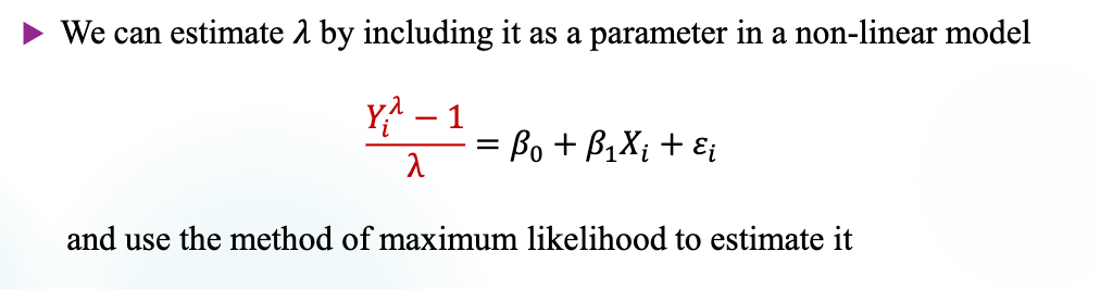
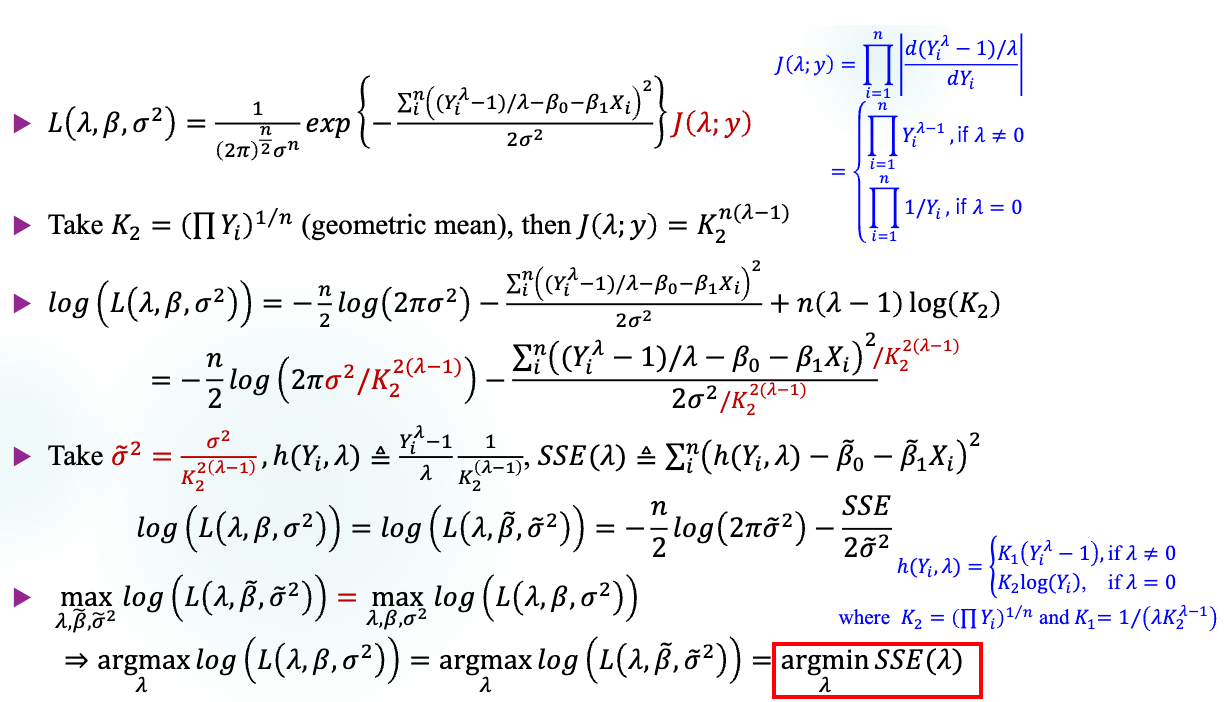
Putting it simple, in order to find the best $\lambda$, we can fix other parameters and optimize $SSE(\lambda)$ only.

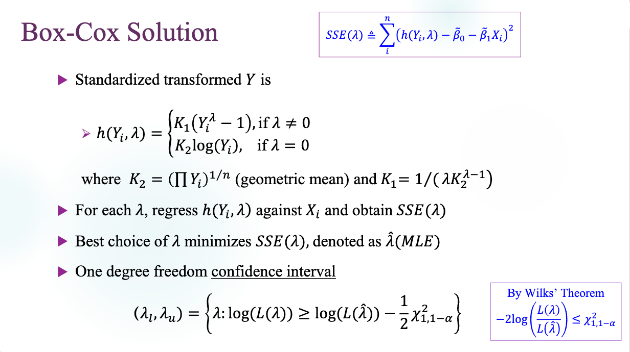
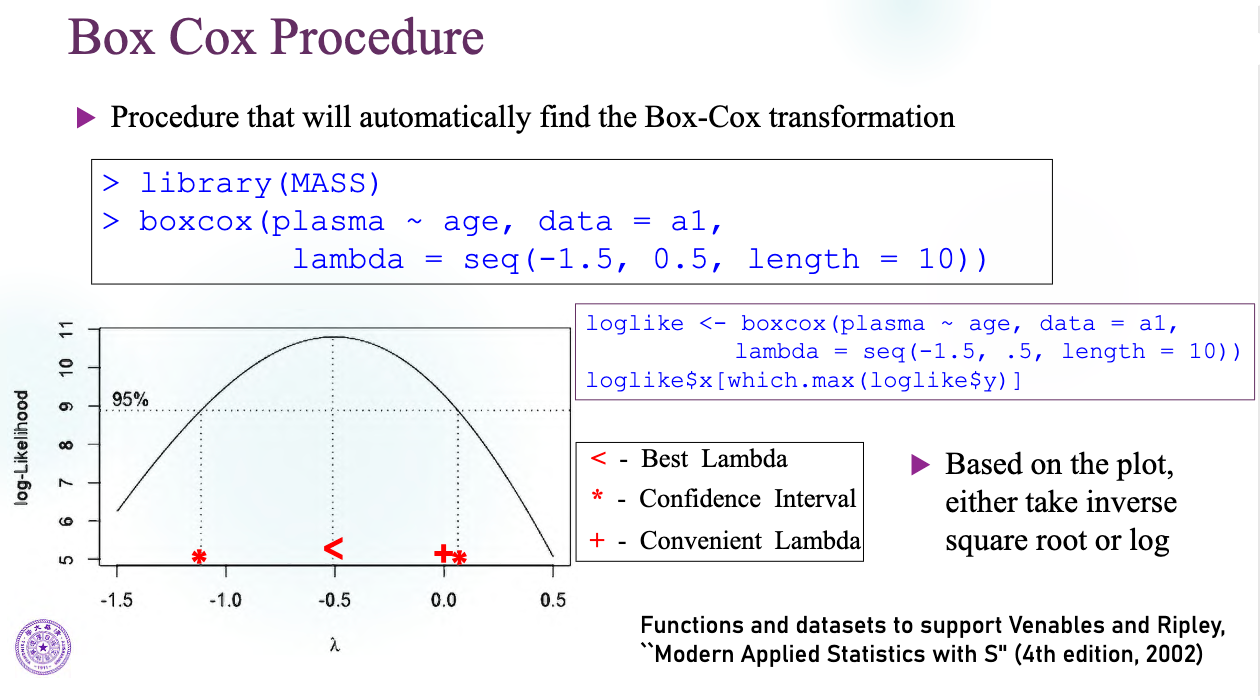
Why we concern the confidence interval:

• Interpretability
• Check if 1 lies in the CI -- that means a linear relationship cannot be rejected.

Other Topics

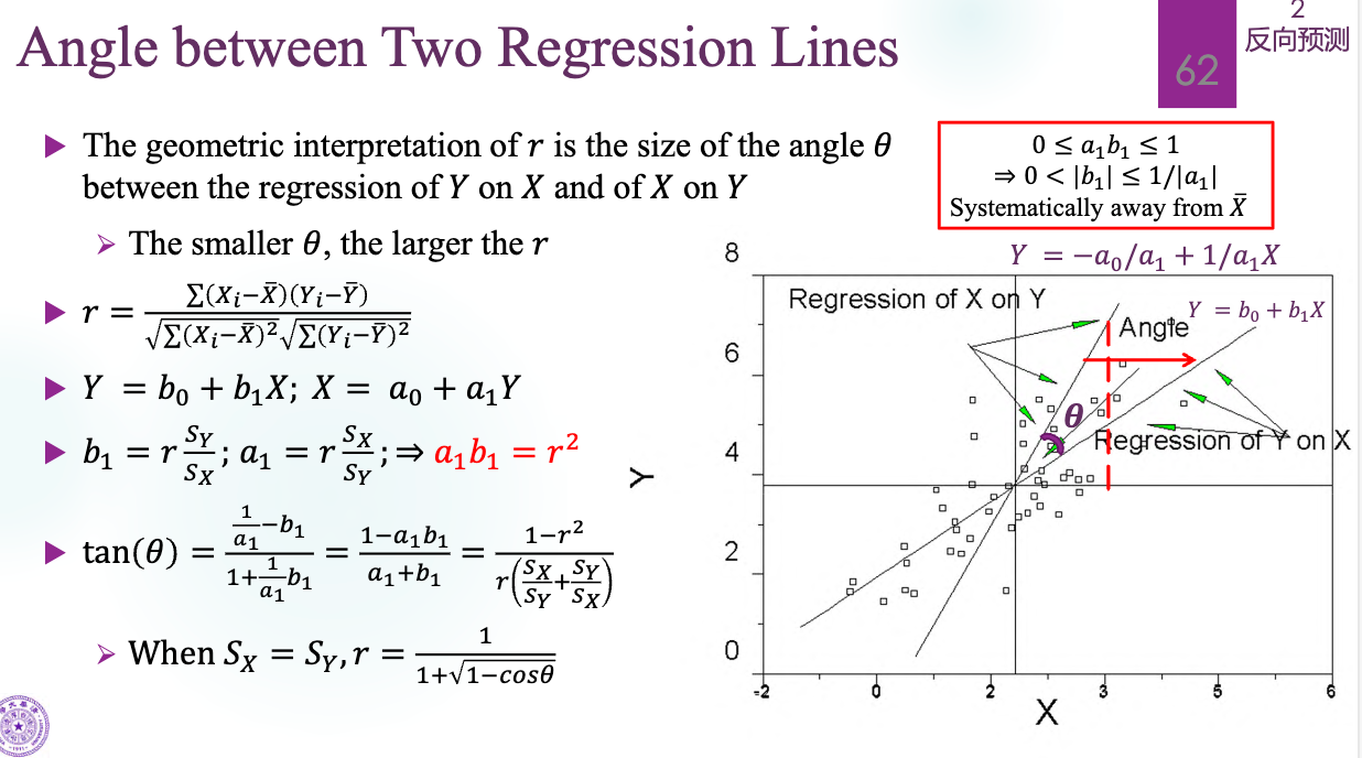
$X\sim Y$ and $Y\sim X$, two fitted lines. Their relationship is: the ratio of their slopes equals to the squared sample correlation.

▶

note on class

第一节课没咋听

失拟 lack of fit，用 GLT 检验

• 区分 full model 和 reduced model
• 三个模型，最细的是 4，1、3 次一级，2 最粗
• 跟上一级比，线性是不是足够
• 以前是检验是不是线性，往下比
• SSE=SSPE+SSLF, pure error, lack of fit, 必须有重复

补救

• power transformation
• 可用 MLE 估计 $\lambda$.
  • pdf 的 transformation
  • 不硬碰硬优化 likelihood function，做变换搞成 LS 之形式解之
• 关注 $\lambda$ 的置信区间
  • 找一个好算的
  • 可解释性
  • 1 在不在区间里，很重要（不做变换）

Regression through the origin （过原点回归）

• 很多东西会崩溃，比如 $\mathrm{Cov}(b,\bar{Y})$ 将不再为零

反向预测

• $\hat{X}_{h}=\frac{Y_{h}-b_{0}}{b_{1}}$.
• 校准
• 为啥不 $X\sim Y$？意义不同
• 两条回归线的夹角越小，相关系数越大

$R^{2}$:

• 啥也不代表，拟合程度、预测能力
• 不能用比较 $R^{2}$ 来评价模型
• 没有因果理解
• Adjusted R2 一样的